By the end of this chapter, students will be able to:

• State the null hypothesis.
• Define an alternative hypothesis.
• Describe hypothesis testing.
• Compare rejecting the null hypothesis and failing to reject the null hypothesis.
• Correlate alpha, the chance of a type I error, and statistical significance.
• Identify a type I error, and propose one method to avoid it.
• Distinguish between statistically significant results and nonsignificant results in a current research article.
• Debate clinical significance given a research article with statistical significance present.
• Analyze statistical information to determine whether statistical significance is present.

• Alpha (α) The significance level, usually 0.05. The probability of incorrectly rejecting the null hypothesis or making a type I error.
• Alternative hypothesis Usually, the relationship or association or difference that the researcher actually believes to be present.
• Clinically significant A result that is statistically significant and clinically useful.
• Fail to reject the null hypothesis Not having enough statistical strength to show a difference or an association.
• Hypothesis An observation or idea that can be tested.
• Hypothesis testing The application of a statistical test to determine whether an observation or idea is to be refuted or accepted.
• Null hypothesis No difference or association between variables that is any greater or less than would be expected by chance.
• Reject the null hypothesis Having enough statistical strength to show a difference or an association.
• Statistical significance The difference observed between two samples is large enough to conclude that it is not simply due to chance.
• Type I error Incorrectly rejecting the null hypothesis.

When you arrive at the clinic at 8:00 AM, you prepare to administer the flu vaccine to patients who show up for one. People are already waiting, and many are wearing business attire. The turnout is much higher than your clinic expected, processing everyone takes longer than expected, and you are the only nurse. The patients are brought into a central receiving area, their background information is collected, and they come to your station for the actual injection. After the first hour, you notice that most of your patients are elderly or unemployed. You realize that it is after now after 9:00 AM. Very few individuals who report outside employment arrive during the hours of 9:00 AM and 5:00 PM. You start to wonder whether employed individuals are less likely to get their flu shots because they cannot come to the clinic during standard business hours, and those who arrived before work may not have been able to stay because of the long delays.

This idea is a hypothesis, an observation or theory that can be tested. You decide to determine whether your observation is actually true. First, you develop your null hypothesis, which states that there is no difference or association between variables that is any greater or less than that expected by chance. (The null hypothesis is represented as H₀.) In this case, the null hypothesis is that there is no relationship between employment status and having a flu shot at your clinic. The alternative hypothesis is usually the relationship, association, or difference that the researcher believes to be present. (The alternative hypothesis is represented as H₁.) In this case, your alternative hypothesis is that employed people are less likely to get a flu shot at your clinic. Hypothesis testing, a fancy term for determining whether you are right, involves using a statistical test to determine whether your hypothesis is true. In this case, when the clinic closes that first night, you decide to collect the information that was gathered on all the patients who arrived at the clinic from 8:00 AM until 9:00 PM that week. Notice that this sample is the group available to you or a convenience sample. You know it is a nonprobability sampling method.

Your statistical analysis of the sample enables you to do one of two things:

• Let’s say the trend of having very few employed patients arriving for flu shots at your clinic continues throughout the day. You may find a statistically significant difference (we’ll explore how to do this later in the chapter) between the number of employed and unemployed people who received the flu shot at your clinic that week. You are then in a position to reject the null hypothesis. You have determined that the difference between the two groups is greater than the difference you might expect to result from chance. Thus, you have evidence of a statistically significant relationship between employment status and receiving a flu shot at your clinic, and you have demonstrated support for your alternative hypothesis.
• On the other hand, let’s say that you collect and analyze the data from the whole week. You find that although there were fewer employed people receiving flu shots between 9:00 AM and 5:00 PM (your initial impression), between 8:00 AM and 9:00 AM, and between 5:00 PM and 9:00 PM, most of the flu shot recipients were employed. In this case, your statistical analysis may not show a significant difference between the number of employed and unemployed people who received the flu shot. You would then fail to reject the null hypothesis. This wording is an important point: You can never “accept” or “prove” the null hypothesis, which is the absence of something. You can only “disprove” it (reject it) or “fail to disprove” it (fail to reject it).

Obstetrics nurses usually understand this slightly confusing concept fairly quickly, so let’s use their clinical experience to create an analogy and help you, too. When a pregnant patient has an ultrasound, the technician attempts to determine the biological sex of the infant by detecting the presence of a penis. The null hypothesis is that there is no penis. The alternative hypothesis is that there is one. If a penis is detected, the ultrasound technician can state that there is one and that the baby is biologically a boy. If a penis is not seen, the technician cannot be sure that there isn’t one; it might be present but undetected (Corty, 2007). As a nurse-midwife, I frequently explain to my patients that if the ultrasound technician told them they are carrying a baby boy, they could consider the report reasonably reliable (but notice that this is still not a probability of 100%). However, I have been in the delivery room when a predicted girl turned out to be a bashful boy. Never overstate what your data allow you to say! You can never say for sure that something does not exist, but the mere presence of what you are looking for can demonstrate that it does. It is also important to remember that statistics is all about probability, and there is always a possibility of an error, so you can never “prove” anything with absolute certainty. The technician who thinks she sees a baby boy could still be wrong.

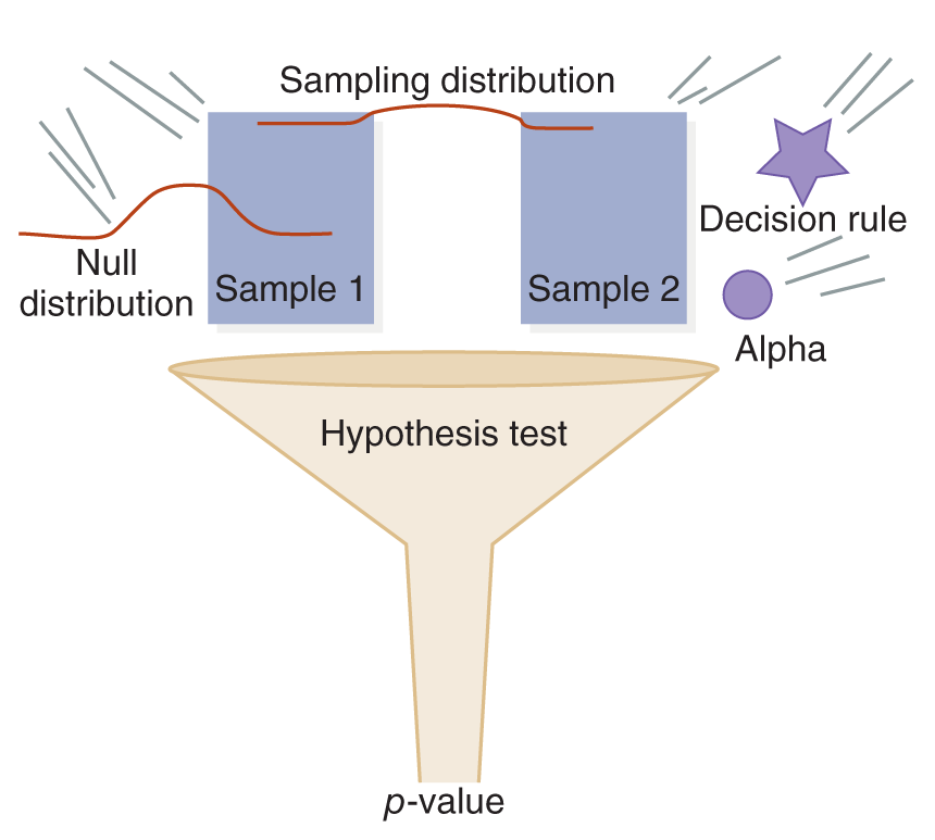
Statistical significance means that the difference you observe between two samples is large enough to conclude that it is not simply due to chance. Statistical significance can be shown in many different ways, but the basic idea remains the same: if you take two or more representative samples from the same population, and there really is a difference between the variables in this population, you would expect to find approximately the same difference again and again. If you have a statistically significant result, you can reject the null hypothesis.

But how do you know whether your result is statistically significant? At the beginning of the study, the researcher selects the significance level, or alpha, which is usually 0.05. This number is simply the probability assigned to incorrectly rejecting the null hypothesis or making what is called a type I error. For example, you conduct a study examining the association between eating a high-fiber breakfast and 10:00 AM serum glucose levels. The null hypothesis is that a high-fiber breakfast is not associated with the 10:00 AM serum glucose levels. The alternative is that it is. You select an alpha of 0.05. This means you are willing to accept that there is a 5% chance that you will reject the null hypothesis incorrectly. If you did so, you would report that eating a high-fiber breakfast is associated with a change in blood sugar levels at 10:00 AM when, in actuality, it is not.

Therefore, the alpha is the preestablished limit on the chance the researcher is willing to take that they will report a statistically significant difference that does not exist. The researcher is willing to say that a statistically significant difference exists right up until the point when the probability of being incorrect is about 5% (alpha = 0.05). An alpha of 0.05 can also be interpreted to mean that the researcher is 95% sure that the significant difference that they are reporting is correct.

Think about this in terms of waking a provider in the middle of the night. You are willing to do that if you are 95% sure your patient has an immediate concern, but you are not so willing to do that if you are only 15% sure that your patient has a pressing issue. The ramifications of being wrong can be substantial at 3:00 AM, no matter what you decide. You may make the call or continue to gather more observations until you are more confident. Remember, all statistical test results are reported as probabilities. No one is absolutely certain that they are correct!

Corresponding to the alpha (which is represented by α) is what statisticians call the p-value. Remember that we started to talk about this concept in Chapter 3. The p-value is the probability of observing a value of a test statistic if the null hypothesis (there is no relationship, association, or difference between the variables) is true. In other words, a p-value tells you the probability of finding your results and the corresponding test statistic if there is no relationship between the variables. This value is also the probability that an observed relationship, association, or difference is due simply to chance. For example, let’s say your study examining the consumption of a high-fiber breakfast and 10:00 AM glucose levels has a test statistic with a p-value of 0.03. Then the probability that the observations in your study would occur if there were no relationship between these variables (or by chance) is only 3%. This result means that you are 97% sure the variables in your study do have a relationship.

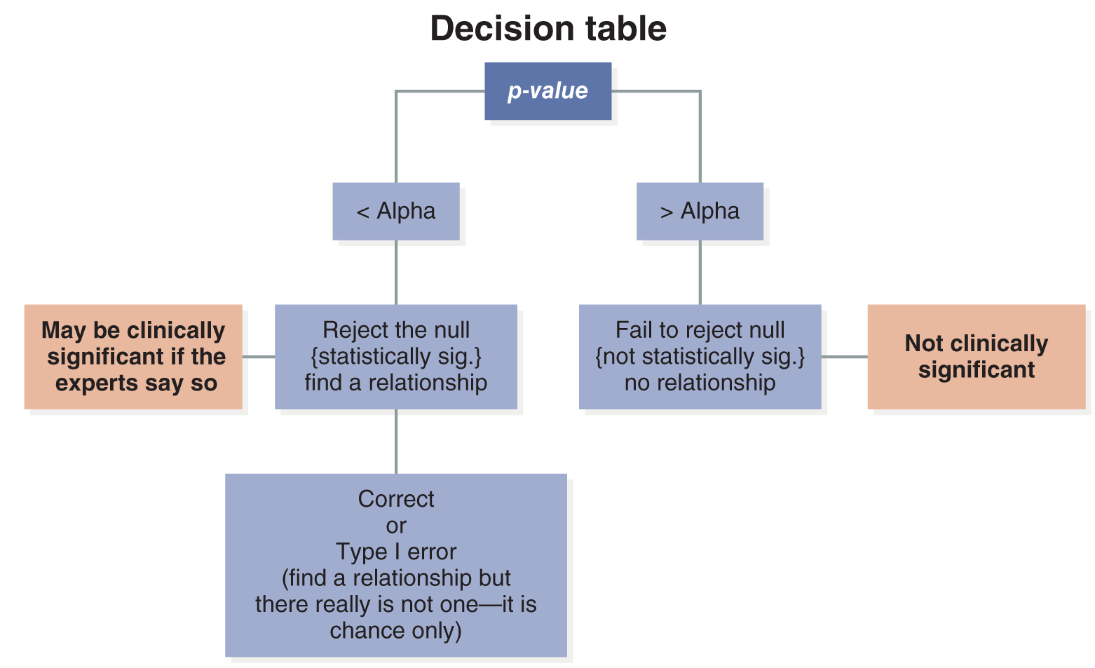
If your study has an alpha of 0.05, it means you are willing to accept up to a 5% chance of making a type I error and reporting that a relationship exists when it is just by chance. Suppose the actual p-value of your test statistic shows you have only a 3% chance of making a type I error (p = 0.03). In that case, you are within error limits that are comfortable for you (5% or less) and can confidently reject the null hypothesis. Rejecting the null hypothesis means reporting a relationship, an association, or a difference between the variables.

So now you know that if the p-value is less than the alpha, you should reject the null hypothesis. However, if the p-value is greater than the alpha, the chance of making a type I error is greater than the level you are comfortable with, and you should fail to reject the null hypothesis. In this case (p > alpha), you would fail to reject the null hypothesis and report that there is no relationship, association, or difference between the variables.

Subtracting the p-value from 1 tells you how sure the researcher is about rejecting the null hypothesis based on the data in that particular study. For example, a p-value of 0.03 means the researcher is 97% sure that the observed relationship is not just due to chance. Sometimes thinking of it this way helps.

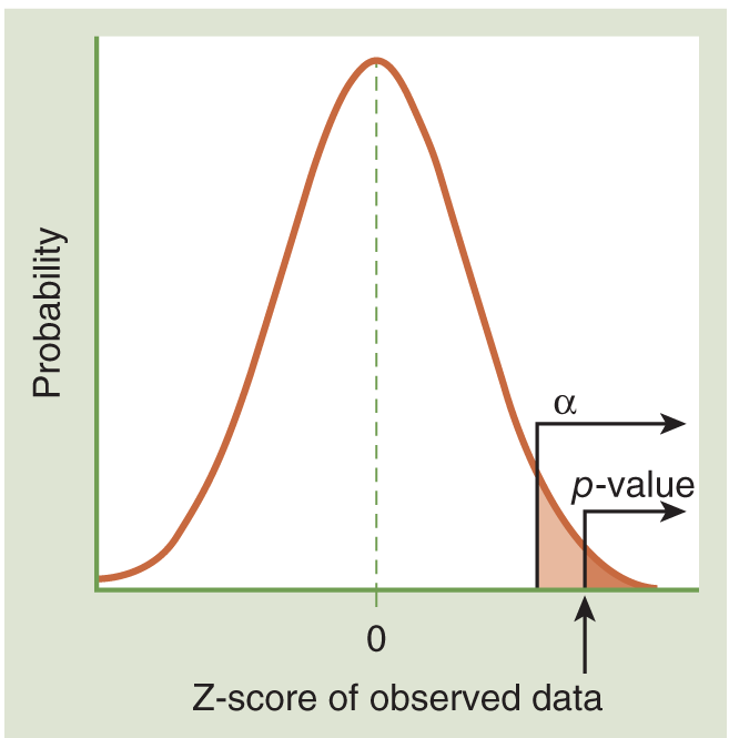
You can see how this looks on the probability distribution in Figure 6-1. A low p-value is way out in the tail of the probability distribution. If it is smaller than your alpha value, then the probability of finding this test result if the null hypothesis is true is smaller than the chance you are willing to take of being incorrect about rejecting the null. This is a graphic illustration of p< alpha, which means you have statistically significant results and should reject the null hypothesis.

Figure 6-1: p alpha.

Statistically significant differences are not the same as clinically significant differences. Clinically significant differences are large enough to indicate a preferential course of treatment or a difference in the clinical approach to patient care. To be clinically significant, a result must be statistically significant and clinically useful. Results that are statistically significant are not necessarily clinically significant, which is a more subjective conclusion.

For example, as a nurse manager, you are approached by the largest chocolate sales team in your region. The team members say that the newest research shows that patients who receive free chocolate from the hospital are discharged earlier. Well, you might be interested in reading the study. The chocolate team conducted a study with 700,000 participants and found that those who were given free chocolate went home on average 2 minutes earlier than those who didn’t. Although you know chocolate makes people feel better, you do not see these statistically significant results as being clinically significant because saving 2 minutes would have very little impact on your unit. Besides, what do the follow-up studies say about tooth decay? In addition, having a very large sample size (700,000 people) in a study might result in statistical significance even though the difference found (the effect size) is actually very small.

Hypothesis Testing in Action

Let’s take it from the top and go step by step through hypothesis testing. The first two steps in a hypothesis test are relatively straightforward, and you already know how to do them. First, you state your null and alternative hypotheses; then, you pick the significance level (alpha) that you wish to have in your study. Remember that typically, the alpha is 0.05, which means that if you find a difference, you are 95% sure it is truly there, not just a chance occurrence.

You also already know that the p-value is going to be compared to the alpha. It is just a probability statement about the actual research results. Just as probability ranges between 0 and 1, so do p-values. The closer a p-value gets to 1, the more likely the related event is (in this case, the conclusion). The closer the p-value gets to 0, the less likely it is. Piece of cake, right?

Choosing which statistical test to perform is more difficult. Which test you choose depends on a number of things, but usually, the most important is how many samples will be compared, how many parts of the population will be estimated, and the format of the variables. We will be talking about all the different statistical tests in the upcoming chapters, but they have a lot in common, so for now, we will speak about them in general terms.

Many tests involve computing a so-called test statistic. One type of test statistic is a Z-score, which is probably all coming back to you from Chapter 3. A Z-score is simply a test statistic that is a standardized measure in a normal distribution. A Z-score tells you how many standard deviations the observation is from the mean. For example, if Z = 3.4, the observation is 3.4 standard deviations above the mean score. If Z = -0.2, then the observation is 0.2 standard deviations below the mean score. Like any other test statistic you compute, a Z-score has a corresponding p-value. We use this p-value to decide to reject or fail to reject the null hypothesis. All test statistics you compute have a corresponding probability or p-value.

From the Statistician

Brendan Heavey

Statistical Testing

What if we want to use the information we collect to make informed decisions? What if we want to use the data to decide how to treat patients or how to predict who will most benefit from new treatments? Questions like these make up the core of hypothesis testing. This “From the Statistician” feature is a little more difficult, but it is at the very heart of the statistical science presented in this text, so try to hang in there with me.

Most statistical testing procedures can be broken down into the five steps shown in Figure 6-2. A hypothesis test is like a funnel that sorts a whole bunch of information in the form of sample data and decision rules and then spits out a single, easy-to-understand p-value. Isn’t it great that there is an easy-to-understand answer after all that work?

Figure 6-2: Hypothesis-Testing Steps.

• State the null and alternative hypotheses.
• Significance level: Determine which alpha to use to determine statistical significance.
• Statistical test: Determine which statistical test to use.
• Compare the distribution of the statistic computed in step 3 to the distribution under the null hypothesis, and report a p-value.
• Decision rule: Decide whether or not to reject the null hypothesis. (Is the sample distribution different enough from the null distribution to say it is more than a chance occurrence?)

Thinking It Through

Dr. Susan Bach

Researchers use statistics to determine whether there is a significant relationship or difference between variables. We sometimes see a relationship or difference, such as when the average age in team 1 is 19, and the average age in team 2 is 20. But how significant is this difference, or are they really about the same? Running a statistical test will tell us if the relationship or difference is statistically significant.

We start with our null hypothesis that there is no difference or relationship between the variables. As nurse statisticians, we hope to reject this null hypothesis and find that, indeed, there is a relationship or difference between two variables; otherwise, we probably wouldn’t bother to do the study. We start by setting our alpha, which is the significance level. Alpha is traditionally 0.05, but we can set it higher or lower depending on the circumstances. Alpha tells us what level of risk we are willing to take that we will incorrectly reject the null hypothesis. For example, with an alpha of 0.05, or 5%, we are willing to take a 5% chance that we will incorrectly reject the null hypothesis (and be 95% sure that if we reject the null, we will be correct in our conclusion).* Remember, if we incorrectly reject the null hypothesis, we are making a type I error.

With every statistical test result, there is an associated p-value. The p-value is the actual probability that our results will be significant. The alpha is the cutoff level. Let’s say we set our alpha at 0.05. If the p-value is equal to or less than the alpha, we reject the null hypothesis and conclude that there is a difference or relationship between our variables. If the p-value is greater than alpha, we retain the null hypothesis (fail to reject the null hypothesis) and conclude that there are no differences or relationships between our variables.

Many students become confused between the alpha and the p-value. The alpha is the significance cutoff that we set ahead of time and compare to the p-value we calculate. The p-value is the actual significance value for the statistical test we calculate with our sample. The preset alpha is the amount of risk we are willing to take that we incorrectly reject the null. Therefore, if our p-value is less than our alpha, we have not gone beyond the level of risk we are comfortable taking.

Computer printouts often list the p-value as significance or Sig. This is the number we must compare to our alpha. Let us look at an example of a chi-square test. Suppose we wish to see if there is a relationship between wearing socks in winter (yes/no) and getting frostbite (yes/no). Our dependent variable is at the nominal level. We decide to set our alpha at 0.05. In this case, if we reject the null, we will be 95% sure there is a relationship between wearing socks and getting frostbite. We are willing to take a 5% risk that we will incorrectly reject the null hypothesis. Remember, the null hypothesis is that there is no relationship between wearing socks and getting frostbite. The alternative hypothesis is there is an association between wearing socks and getting frostbite. We use our statistical software to calculate a p-value for our chi-square statistic. Then, we look at the p-value and compare it to 0.05 (our alpha) to see if it is less than or more than the alpha. Let’s imagine that our p-value is 0.02. In this case, we reject the null hypothesis and conclude that there is a relationship between wearing socks and getting frostbite. Another way of looking at this is that now we can be 98% sure that our results are significantly different. Our p-value indicates that the risk of incorrectly rejecting the null is only 2% (100% - 2% = 98%).

One last thing: some students find it challenging to determine whether the p-value is more than or less than the alpha. One trick I find helpful is to convert both the alpha and the p-value to a percentage, which eliminates the confusion created by the decimal point. To do this, you just multiply both the alpha and the p-value by 100. For example, if our alpha is 0.05, we multiply by 100, which becomes 5%. If our p-value is 0.04, we multiply by 100, and it becomes 4%. We can easily see that 4% is less than 5%. So we know that this p-value is less than our alpha, and we reject the null hypothesis and conclude that we have a statistically significant result. If instead our p-value were 0.4, we would multiply it by 100, and it would become 40%. Now we can quickly see that 40% is more than 5%. Therefore, we would fail to reject our null hypothesis and conclude that there is no relationship between wearing socks and getting frostbite. Sometimes little tricks like this can help you avoid a mistake.

*This is the basic idea, but statistically, the full explanation is more complicated than this. This is another idea you can explore further in a future statistics class!

Let’s look at those p-values graphically again. Figure 6-3 is a picture of a hypothesis test using the normal distribution. We can see that the area under the normal curve varies when drawing vertical lines at different Z-scores. This area is what we need to know to report p-values. In this case, 2.5% of the probability can be found in each tail of the distribution. (This is how your alpha is distributed when you have a two-tailed test, which involves a nondirectional alternative hypothesis—for example, when the researcher believes there is a relationship between the independent variable and the dependent variable but isn’t sure if the change in the independent variable will be associated with an increase or decrease in the dependent variable.) The area underneath the normal curve, above the horizontal axis and past the vertical lines, totals 0.05. This is your alpha value (0.025 in each tail). These vertical lines also represent the Z-value that corresponds with these probability levels. A Z-score of 1.96 corresponds to an alpha of 0.05 in a normal distribution. In this case, the test statistic you computed was a Z-value of 2, greater than 1.96 (the cutoff for statistical significance on the horizontal axis), so our statistical test falls further out into the upper tail of the null distribution. Whenever that happens, we say that the observed data are significantly different from what we would expect under the null distribution (or if the null distribution were true).

Figure 6-3: The Normal Curve.

This should make sense conceptually. As your observations get farther and farther away from the center of the data (mean), two things happen:

• The Z-score (test statistic) gets pushed farther and farther into the tails of the statistical distribution.
• The p-value associated with that Z-score (test statistic) gets smaller and smaller.

And as you already know, the smaller the p-value is, the less likely it is that this observation is due simply to chance, and the more sure you can be that the difference you found is actually there.

We need to see if our p-value is less than or greater than alpha to apply our decision rule. In our last example, the probability of observing the statistical results we found if the null hypothesis were true (p-value) is low and, in this case, less than alpha. Because p< alpha, we conclude that this observed difference is not just due to sampling error or chance; we reject the null hypothesis and report that a difference, association, or relationship exists between the two variables. If the p-value were greater than alpha, we would decide to fail to reject the null and report that there is no relationship, association, or difference between the variables.

Whew! That was a tough one, but you should now be starting to understand the link between test statistics and p-values. This concept directly transfers from Z-scores to other test statistics such as T-scores, F-scores, and chi-square scores. All of the calculated test statistics have a corresponding p-value. You have to look at it to determine if there is a statistically significant difference and what conclusion you should draw about the null hypothesis. The different tests differ in the types of data involved and the quantities being estimated, but they work on this same principle. If the p-value associated with the computed test statistic is less than the alpha value chosen in the decision rule, you should reject the null hypothesis.

Thinking It Through

In this chapter, we are going to start building a decision tree (see Figure 6-4). We will expand on it in the next chapter. This tree is a handy way to start breaking down the decisions you are making during hypothesis testing.

Figure 6-4: Decision Table.

When you have to decide what to do about the null hypothesis, you always start at the top of the decision tree. What is your p-value?

Then you compare the p-value to alpha. If the p-value is < alpha, start down the left side of the decision tree. That means you should reject the null and conclude that there is a statistically significant relationship between the variables. If you keep going on the same side of the tree, you will find that your conclusion is either correct or it is a type I error. The side branch shows you that if you are on this side of the decision tree, your results may also be clinically significant if the experts in the field reach this conclusion.

When you examine the p-value, if you find it is greater than alpha, you head down the right side of the decision tree instead. In this scenario, you would fail to reject the null and conclude that there is no statistically significant difference and find no relationship between the variables. The branch from this side of the tree reminds you that there are no clinically significant results once you are on this side of the tree because there are no statistically significant results.

This decision tree is really handy because once you have established which side of it you are on, you just stay on that side. You can’t jump the tracks to the other side. Sometimes questions will start in the middle of the track, such as telling you the study reported a statistically significant difference in the average heart rate of spouses. At that point, you would find yourself in the middle of the left side of the tree, where it says “Reject the Null” (statistically significant). If you are then asked what this means about the p-value, you can upwardly follow that side of the tree and see that the p-value is less than alpha. If instead, you are told the conclusion was an error and asked what type of error it would be, you would follow the tree down and see that when you have statistically significant results and there is an error, it would be a type I error. When we add to the tree in the next chapter, you will see how this can help you think through problems and not start to confuse the ideas in your head.

Try using the tree to help answer these questions:

• The study reports a p-value of 0.18. What would you conclude about the null hypothesis? Because p > alpha, you are on the right side of the decision tree, so you would fail to reject the null.
• Your study rejected the null, but you found this to be a type I error upon further evaluation. What do you know about the p-value in the original study? Because you are at the bottom of the left side of the tree, you have to stay on that side. You will find out that when a type I error was made in the original study, p < alpha, and the null was rejected. Unfortunately, it was not correct, and a type I error was made.
• Your study reports a p-value of 0.24. Is it clinically significant? In this case, p > alpha, so there is not a statistically significant difference. You follow the branch of the right side of the tree over and see it that cannot be clinically significant because it is not statistically significant.

You have just completed the chapter! The concepts are getting pretty technical, but keep reviewing and practicing to maintain and enhance your knowledge. Now we can review some of the important concepts in this chapter.

A hypothesis is an observation or idea that can be tested. The null hypothesis states that there is no relationship, association, or difference. The alternative hypothesis is the opposite of the null: there is a relationship, association, or difference (what you actually think is true). Hypothesis testing involves using a sample to determine whether your hypothesis is true.

When you reject the null hypothesis, you have found statistical support for your alternative hypothesis. When you fail to reject the null hypothesis, you do not have enough statistical strength to say there is a relationship or an association. There may not really be a relationship, or you may not have a sample that is large enough. You can never accept the null hypothesis. If you reject the null hypothesis incorrectly, it is a type I error.

Statistical significance means that the difference you observed between two samples is large enough not to be simply due to chance. To determine statistical significance, you need to identify the alpha’s significance level, which is usually 0.05. If your p-value is less than alpha, you have statistical significance. For something to be clinically significant, a result must be statistically significant and clinically useful.

This chapter presented a lot of information, but if you are able to grasp these concepts, you are doing well! However, if it still seems a bit murky, don’t worry. We will continue to work with these ideas and reinforce them as you build your knowledge!

1. For review questions 1-5, you are conducting a study to determine whether there is an association between years worked in nursing and salary earned. Write the null and alternative hypotheses.

   Show Answer

2. If you find a p-value of 0.09, what would you conclude?
3. If you find a p-value of 0.03, what would you conclude?

   Show Answer

4. If you reject the null hypothesis, what type of error is it if you are wrong?
5. If your p-value is 0.03, is the conclusion clinically significant?

   Show Answer

6. For review questions 6-15, you are conducting a study to determine whether there is an association between a positive toxicology screen for Rohypnol (flunitrazepam) and signs of sexual assault in a sample collected from three large emergency rooms throughout your state. Write the null and alternative hypotheses.
7. As the primary investigator in this study, you realize your results may be utilized in a courtroom setting, and you do not want to make a type I error. Would you prefer an alpha of 0.05, 0.10, or 0.01?

   Show Answer

8. Your study includes all individuals who arrive in the three emergency rooms with a diagnosis of sexual assault over a 1-month period. This is what type of sample?
9. You conduct the study with an alpha of 0.05, and your test statistic has a p-value of 0.02. What do you conclude?

   Show Answer

10. You get the consent of the study participants and conduct a follow-up study in which you interview the family members of the individuals included in your study. This is an example of what type of sampling?
11. You ask the family members to describe the appearance and manner of the individuals who were assaulted when they were taken to the emergency room. Is this a qualitative or quantitative measurement?

    Show Answer

12. You also collect a measure of the patient’s sedation provided by the sexual assault nurse examiner. It is coded as follows: 0 for no sedation, 2 for mild sedation, 5 for moderate sedation, 7 for heavy sedation, and 10 for unable to arouse. This variable can be analyzed as being at what level of measurement?
13. In your sample of 45 patients, 10 showed no signs of sedation, 12 were mildly sedated, 3 were moderately sedated, 13 were heavily sedated, and 7 were not arousable. What percentage was mild or moderately sedated?

    Show Answer

14. What is the median level of sedation?
15. You are putting together a grouped frequencies table and want to categorize these responses as patients showing signs of sedation and those not showing signs of sedation. How many patients showed signs of sedation? What percentage of your sample is this?

    Show Answer

16. Write an appropriate null hypothesis.
17. Write an appropriate alternative hypothesis.

    Show Answer

18. If HPV infection is measured as not infected, infected with a low-risk strain, or infected with a high-risk strain, at what level of measurement is this variable?
19. If the presence of cervical cell abnormalities is measured as biopsy results being positive or negative, at what level of measurement is this variable?

    Show Answer

20. If cervical cell abnormalities are measured as biopsy pathology results of negative, CIN I, CIN II, CIN III, or cancer in situ (CIS) (these are progressively worse levels of abnormality), at what level of measurement is the variable?
21. In your state, 30% of cervical biopsies are negative, 40% are CIN I, 20% are CIN II, 5% are CIN III, and 5% are CIS. For your study, one lab is randomly selected in each of 10 regions of the state, and at each of these labs, 120 biopsy results are randomly selected and reviewed. What type of sample is this?

    Show Answer

22. Is it a probability or nonprobability sample?
23. In one of the random samples of 120 biopsies, 16 are negative, 42 are CIN I, 30 are CIN II, 22 are CIN III, and 10 are CIS. In the same sample, 1 person is HPV negative, 87 are HPV positive with the low-risk strain, and 32 are HPV positive with the high-risk strain. What percentage of your sample is CIN II or greater?

    Show Answer

24. What percentage is not infected with a high-risk strain?
25. What percentage has an abnormal cervical biopsy?

    Show Answer

26. What is the median biopsy result?
27. What biopsy result is the mode?

    Show Answer

28. Can you determine the mean biopsy result? Why or why not?
29. What is the median type of HPV infection?

    Show Answer

30. What is the mode for the type of HPV infection?
31. The study reports the association between the type of HPV infection and cervical cell abnormalities has a p-value of 0.06. If the alpha for the study is set at 0.05, what should the researcher conclude regarding the null hypothesis? Why?

    Show Answer

32. What is the prevalence of HPV infection in this sample?
33. If instead of an alpha of 0.05, the researchers decided to set this pilot study’s alpha at 0.10, what would the researcher conclude about the null hypothesis (p = 0.06)?

    Show Answer

34. If the researcher rejects the null but does so in error, what type of error could the researcher be making? What does this type of error mean?
35. If the researcher does find a statistically significant difference, does this mean it is a clinically significant difference?

    Show Answer

36. If the researcher reports an alpha of 0.05 and a p-value of 0.09, are the results clinically significant? Why or why not?
37. Write what you would conclude about the null hypothesis with the following results at the two different levels of alpha:

    Study	p-Value	Alpha = 0.05	Alpha = 0.10
    A	0.0647
    B	0.912
    C	0.1567
    D	0.0211
    E	0.081

    Show Answer

38. Refer to the table in review question 37. If the researcher is incorrect about the decision made regarding the null hypothesis, which studies could be a type I error at an alpha of 0.05? Why?
39. Refer to the table in review question 37. If the researcher is incorrect about the decision made regarding the null hypothesis, which studies could be a type I error at an alpha of 0.10? Why?

    Show Answer

40. Does increasing the alpha increase or decrease the risk of a type I error?

1. H₀: There is no relationship between years worked and salary earned.

H₁: There is a relationship between years worked and salary earned. (Or you could write, “More years worked is related to a higher earned salary.”)

3. Reject the null. The p-value is significant; therefore, you conclude that there is a relationship between years worked and salary earned.

5. You do not know. It depends on the clinical judgment of the experts in clinical care. You may be one of them!

7. Alpha of 0.01

9. Reject the null. There is an association between a positive toxicology screen for Rohypnol and signs of sexual assault.

11. Qualitative

13. 15 ÷ 45 = 33.3%

15. 35 ÷ 45 = 77.7%

17. There is a relationship between the strain of HPV infection and cervical cell abnormalities.

19. Nominal

21. Two-staged cluster sample

23. 62 ÷ 120 = 52%

25. 104 ÷ 120 = 87%

27. CIN I

29. Low risk

31. Fail to reject the null; p >alpha

33. Reject the null; p< alpha

35. No, in addition to being statistically significant, experts in the field must also support the argument that it is a clinically significant difference.

37.

39. A, D, E—in order to make a type I error, you must reject the null incorrectly.

Answers to Data Analysis Application questions can be found in the Instructor Resource package accompanying this text.