By the end of this chapter, students will be able to:

• Identify the conditions under which regression is an appropriate statistical technique.
• Compare and contrast linear regression, multiple regression, and logistic regression.
• Explain how quantifying an association with a regression equation helps a researcher infer or predict future events.
• Use regression coefficients to interpret how a change in the independent variable affects the predicted value of the dependent variable.
• Contrast positive and negative regression coefficients.
• Discuss when reporting an adjusted R-squared is more appropriate.
• Interpret the statistical computing program output utilizing multiple regression, determine whether the model and the independent variables are significant, and interpret these results in statistical terms and in plain English.
• Critique an article from current nursing research that utilizes a regression technique, determine whether statistical significance is present, and debate whether clinical recommendations should be made.

• Adjusted R-squared Value reported to avoid overestimating the percentage of variance in the outcome explained by the model, such as when there is a large number of independent variables with a relatively small sample size.
• Linear regression Technique for analyzing the relationship between a single independent variable and a single interval- or ratio-level dependent variable, enabling the researcher to make a prediction about a future outcome based on the research data included in the analysis.
• Logistic regression Method for analyzing the relationship between multiple independent variables and a single dependent or outcome variable when the outcome is binary (has only two categories).
• Multicollinearity A problem that exists when two independent variables (predictor variables) are closely correlated in a regression model.
• Multiple regression A statistical method used to look at the relationship between a dependent variable and multiple independent variables to develop a prediction equation based on the research data included in the analysis.
• Odds ratio (OR) The odds or probability of the outcome occurring divided by the odds or probability of the outcome not occurring.
• R-squared change The change in the percentage of the variance in the outcome variable (R²) that is explained by the model with the addition of another independent variable.
• R-squared value (R²) The percentage of the variance in the dependent or outcome variable that is explained by the model.
• Regression A statistical technique that allows the researcher to make a prediction about a future outcome based on the research data included.
• Regression coefficient The b value, which tells you the rate of change in the outcome or dependent variable with a one-unit increase in the corresponding independent variable.
• Residual The amount of prediction error in a regression equation.
• Standard error of the estimate The average amount of error there will be in the predicted outcome using a model.

It is one thing to recognize statistically significant relationships and another to be able to use that information to begin the process of inferring or predicting future events. In order to do that, we first need to quantify the association. Let’s look at an example. Most obstetric nurses have read the literature showing a significant relationship between smoking and fetal weight. This is helpful knowledge to have for our pregnant patients. However, if you have a patient who is smoking 10 cigarettes a day and really doesn’t want to quit, she may not think smoking 10 cigarettes a day will have that much of an impact on the size of her baby. Just being able to tell her there is a statistically significant correlation between smoking and fetal weight may not be enough. You are going to need to use more statistics before you can convince this patient that it is important for her to quit smoking.

You know that correlations measure the strength of associations; now we want to be able to quantify that association, which involves one of my favorite statistical techniques, called regression. No, we are not all going to take a moment and relive childhood memories. This is math, remember, but it can still be fun! Regression happens to be a favorite test of mine for one basic reason: developing an accurate regression equation is the first step in being able to predict future events. It is like being a psychic—but this time your predictions should actually be true!

Of course, there isn’t just one kind of regression analysis, so let’s start with the most basic, although not one that is used that often in the literature. You need to understand the basics of linear regression before you understand the more complex types of regression, so it is a good place to begin.

Linear regression looks for a relationship between a single independent variable and a single interval- or ratio-level dependent variable. (You can sometimes use this technique when you have ordinal-level dependent variables as well, but it gets a little more complicated.) Once the temporality of the relationship is established, you can then make an inference or a prediction about the future value of the dependent variable at a given level of the independent variable. In the fetal weight example, you might use linear regression to see the relationship between the number of cigarettes smoked each day and fetal weight. Maybe knowing, for example, that for every five cigarettes a day a patient doesn’t smoke, her baby will weigh about a half a pound more will help motivate your pregnant patient to decrease her cigarette smoking.

From the Statistician

Brendan Heavey

Statistics, Jerry Springer Style: Now Let’s Look at Some Relationships That Aren’t Functional!

Regression is a method that allows us to examine the relationship between two or more variables. You may recall another way of exploring the relationship between two variables from earlier in life when you first learned to graph a line using the formula Y = mX + b. Remember what all these letters represent:

Y is the dependent variable and is displayed on the vertical axis.

X is the independent variable and is displayed on the horizontal axis.

M is the slope and represents the amount of change in the Y variable for each unit change in the X variable.

b is the Y-intercept, and it tells us the value of Y when the line crosses the vertical axis (X = 0).

In this relationship, the value of the variable Y varies according to the value of X based on the values of two constants, or parameters. If you know the values of m, X, and b, you can solve for the value of Y exactly. Let’s look at an example. In the graph shown in Figure 12-1, you can see three functional relationships between the total cost of three different types of treatment for minor wound infections in June. Treatment 1, outpatient treatment, is cheaper per unit, so there is a more gradual rise in overall cost for each additional treated case. Because all three treatments pass through the origin, their Y-intercepts are all 0. In fact, the only differences between these three lines are their slopes. Their equations are:

Figure 12-1: Relationship Between Total Cost and Number of Patients Treated (Functional Relationship).

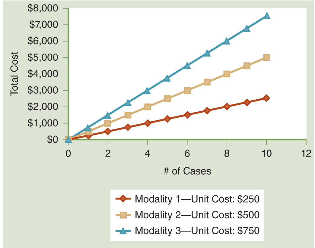
Treatment 1 (outpatient)—$250/case: Y = 250 X

Treatment 2 (inpatient medical treatment)—$500/case: Y = 500 X

Treatment 3 (same-day surgical treatment)—$750/case: Y = 750 X

This math is all well and good, but things rarely work out this nicely in nature. The problem that usually occurs is that the relationship between most variables, just like the relationship between many people, is not functional. Can you guess what term best describes the relationship between almost all variables? Why, statistical, of course! You see, the difference between a functional relationship and a statistical relationship is that a statistical relationship accounts for error.

As it turns out, accounting for error is a very difficult task. We rarely, if ever, know how error is distributed around a mean value, so we usually have to make a few assumptions to allow us to make sense of our data.

In this text, we are doing our best to keep things simple and give you a basic introduction to regression, so we will stick with one of the most basic regression models available, namely, the normal error regression model. In this model, our most basic assumption is that the error we model is normally distributed around the mean of Y. This is okay to do, especially as our sample size is increased. Do you remember why? It is because of the central limit theorem. Because the distribution of the sum of random variables approaches normal as the number of variables is increased, and as our sample size increases, the amount of random error increases, we can assume that the distribution of this random error approaches normality. It is okay to make this assumption as long as you have a large enough sample. It is important to note that a few other assumptions are used in the normal error regression model, but they are beyond the scope of this text and most aspects of life.

So now let’s look at what a statistical relationship or statistical model looks like. Here is the definition of the normal error regression model:

Y_i = β₀ + β₁X_i + ε_i

In this model, there are three variables and two parameters (one more than the functional model you just saw). Here is what each of these terms means:

Y_i: The value of the dependent variable in the ith observation

X_i: The value of the independent variable in the ith observation

ε_i: The normally distributed error variable

β₀ and β₁ are parameters, just like the slope, m, and the Y-intercept (b) were in the functional relationship earlier.

Let’s say we now have a little more information on treatment 1 (outpatient management) from our previous example. In this case, although there was an exact functional relationship between the number of cases and total cost, when we look at the relationship between unit cost and time, it looks like this:

Cost of Treatment 1 Throughout the Year
January	$118
February	$150
March	$165
April	$205
May	$215
June	$253
July	$276
August	$289
September	$310
October	$325
November	$332
December	$362
Average	$250

There is not an exact functional relationship. In fact, the unit cost is increasing over time, but the amount of each increase is different each month. The increase in cost per month varies according to a few different factors, but you can see that if we graph these data, the trendline shows that unit cost is increasing, on average, by $21.72 per month (see Figure 12-2).

Figure 12-2: Unit Cost by Month for Treatment 1.

Notice that you can see the error in this relationship. The trendline shows you a functional relationship that is buried inside the statistical relationship. The functional relationship is exactly quantified by two parameters and two variables:

Y = 21.72 X + 108.82

The statistical relationship adds a third variable (error, ε), which allows the points on the graph the freedom to vary around this functional relationship because statistical relationships are never exact:

Y = 21.72 X + 108.82 + ε

Linear regression plots out the values of the dependent variable (i.e., fetal weight) on the y-axis and the values of the independent variable (i.e., daily number of cigarettes) on the x-axis to find the line to illustrate the relationship between the two variables best (see Figure 12-3).

Figure 12-3: Fetal Weight at Various Levels of Daily Cigarette Consumption.

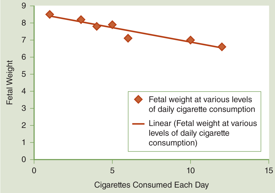
Assuming there is a linear relationship (you can see how a trendline is not exactly on the points of data, but the points follow it pretty closely or in a linear fashion), this line can then be used to make predictions about the future value of the dependent variable at the different levels of the independent variable. The difference between where the points of data actually fall and where the line predicts they will fall is something called a residual, or the prediction error, which is discussed further in the next “From the Statistician” feature. The lower the amount of residual, the better the line fits the actual data points.

The slope of the trendline tells how much the predicted value of the dependent variable changes when there is a one-unit change in the independent variable. In our example, the slope of the line would tell us how much the predicted fetal weight would drop with the consumption of an additional cigarette each day. Seems simple enough, right?

Unfortunately, life is rarely so simple, and statistics has to keep up with it. (And you thought statistics was what made life complicated!) Very rarely is there only one independent variable we need to consider, which may leave you asking: What do you do when you want to predict how two or more variables will affect the dependent or outcome variable? For example, the length of the pregnancy and the number of cigarettes smoked each day both affect fetal weight. You would not want to predict fetal weight with just one of these independent variables; you would want to include both. How can you make an accurate prediction in this situation? (No, no, don’t use the crystal ball. . . .) You just need to use another statistical test called multiple regression.

So let’s go back to the example of studying fetal weight. Multiple regression lets us take the data we have measuring months pregnant (independent variable number 1 or X₁) and the number of cigarettes smoked (independent variable number 2 or X₂) and see how these variables relate and affect the outcome, which is fetal weight (dependent variable or Y). Using this example, the relationship can be expressed in an equation like this:

Y_i = a + b₁X₁ + b₂X₂ + e

Now I know many of you just looked at this equation and started to think, what on earth does this equation mean? Don’t panic. Let’s break it apart.

Y_i is just the value of your dependent variable, in this case, how much the fetus weighs.

The value of a is what is called the constant, or the value of Y when the value of X is 0. In our example, this would be the value of Y or fetal weight when the patient is not yet 1 month pregnant and has not smoked any cigarettes. Obviously, there would still be some fetal weight, although in this example, a is probably going to be a very small number.

b₁ is the value of the regression coefficient for our first independent variable. It is the rate of change in the outcome for every one-unit increase in the first independent variable. In our example, it is how much we would expect fetal weight to increase for each additional month of pregnancy.

X₁ is the value of our first independent variable, or, in this example, how many months pregnant the patient is at the time of measurement.

b₂ is the value of the regression coefficient for the second independent variable. It is the rate of change in the outcome for every one-unit increase in the second independent variable. In our example, it is how much change we would expect in fetal weight when one additional cigarette is smoked every day. In all likelihood, the value of b₂ would be negative in this example because increases in daily cigarette consumption usually lower fetal weight. If the value of the regression coefficient is negative, an increase in the corresponding independent variable produces a decrease in the dependent or outcome variable, such as an increase in cigarette consumption producing a decrease in fetal weight.

From the Statistician

Brendan Heavey

What Is a Residual?

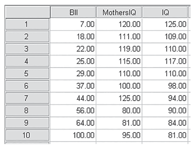
Consider the following data, which show the results of a survey that collected IQ levels for a series of patients with elevated blood lead levels (BLLs):

Obs.	BLL (mcg/dL)	IQ
1	7	125
2	18	109
3	22	110
4	25	117
5	29	110
6	37	98
7	44	94
8	56	90
9	64	84
10	100	81

Now, you can see in Figure 12-4 what these data look like when we graph them. Let’s look at this model a little more in depth. To do so, we’ll need two definitions:

Figure 12-4: IQ Versus BLL.

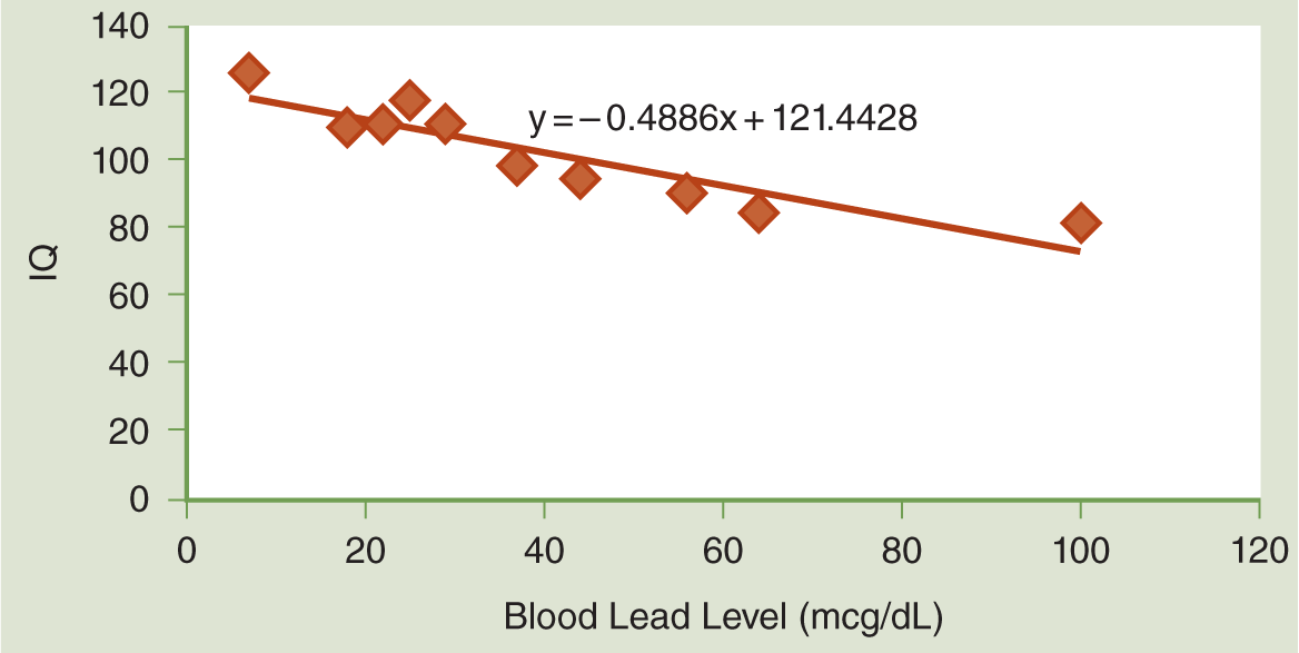
• We refer to the fitted value of our regression function (or the inferred value of the dependent variable) at a particular X value as Ŷ(pronounced Y-hat). Because the formula for our regression line is Ŷ= -0.4886 X + 121.4428, if we are interested in the fitted value at an X of 7, we solve for Ŷlike this:

Ŷ= -0.4886(7) + 121.4428

Ŷ= -3.4202 + 121.4428

= 118.0226

This means that at a BLL of 7, our regression model infers an IQ of 118.0226 on the y-axis.

• We refer to the distance between the actual observed value and the regression line as a residual, which is usually labeled using the Greek symbol ε. On a graph, it looks like Figure 12-5.

Figure 12-5: Residuals for Figure 12-4.

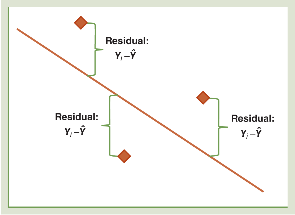
In this example, the fitted regression function equals 118.02 at an X of 7. Now, look at the data we observed to come up with this regression line. The observed value at an X of 7 was 125. Therefore, our residual value at an X of 7 is:

ε= 125 - 118.02 = 6.98

Let’s look at the data from our example and calculate the residuals for our model. Plug in each of the Xs to solve for Ŷ, and then subtract from the actual observed value to get the residual:

Observation	Blood Lead Level (mcg/dL)	IQ (Yi)	Ŷ	Residual
1	7	125	118.02	6.98
2	18	109	112.65	3.65
3	22	110	110.69	0.69
4	25	117	109.23	7.77
5	29	110	107.27	2.73
6	37	98	103.36	5.36
7	44	94	99.94	5.94
8	56	90	94.08	4.08
9	64	84	90.17	6.17
10	100	81	72.58	8.32
			Sum	0

Notice that if you sum the residuals, you get a total of 0. This is always true for the normal error linear regression model.

Finally, it is important to point out the distinction between residuals and error. Remember the normal error regression model:

Y_i = β₀ + β₁X_i + ε_i

It is really easy to confuse the final variable in this model, which represents the error, with residuals. Remember, residuals are a real construct. They are easily calculated from observed data. They represent the observed error. The error term in the model is more abstract. It represents all errors from the entire model, which has a much larger range than our observed data.

Last, there is always an error term in statistics, and in this equation, it is represented by the e. Just as there are no perfect people, there are no perfect estimates. The e just acknowledges that these statistical procedures are estimates taken from a sample, not the parameters you would find in a population model.

So if we wanted to put the previous equation into plain English using our example, we would say:

Fetal weight = a baseline value + an amount related to the length of the pregnancy + an amount related to the number of cigarettes smoked (probably negative) + a certain amount of error

Now hopefully that makes a little more sense.

Once you put in the data you have about the duration of the pregnancy and the number of cigarettes smoked, assuming this is a good regression equation, you should be able to predict an accurate fetal weight. For example, after we compute the regression equation, we determine the following:

Y = 0.25 + 0.79X₁ - 0.15X₂ + 0.5

A patient comes into your unit who is having some preterm labor at 7.5 months. She reports smoking 10 cigarettes a day. You might be concerned because you would predict the current fetal weight to be only 5.18 pounds.

Y = 0.25 + 0.79(7.5) - 0.15(10) + 0.5

Y = 5.175 pounds

Given that information, you might anticipate transferring the patient to a tertiary care facility if you are unable to stop the preterm labor.

Now the next question becomes: How do you know if you have a good regression equation? See, I knew you were going to ask that! Let’s look at some computer output to answer that question. There is another piece of good news when it comes to regression analysis, which is that you are not going to do any of the calculations yourself. We are going to make the computer do all the hard work, and then we are going to look at the results and see what we have figured out. However, for those of you who like to see the math to help understand the concept, check out the “From the Statistician” feature, where you can learn to calculate the regression coefficients manually.

From the Statistician

Brendan Heavey

Calculating Regression Coefficients (Parameter Estimates)

Regression coefficients (parameter estimates) can be calculated in many ways; the method you probably will choose is to use some computer software package to spit them out. However, I think it is an important exercise to see just what that computer package is doing behind the scenes.

Remember, the normal error simple linear regression model we have been looking at thus far is:

Y_i = β₀ + β₁X_i + ε_i

This model represents how variables and parameters interact in a population. The true values for the parameters β₁ and β₂ are never really known. However, when we sample real data from a population, we can come up with very good estimates of what these parameters are, given a few reasonable assumptions, by using the following two equations. Notice that we need the result of the first equation to solve the second equation:

These equations are called the normal equations and are derived using a process called ordinary least squares.

To calculate these parameters, the first thing we do is find the denominator in the equation for b₁:

This denominator is an example of a very important concept in statistics called a sum of squares, which is calculated by subtracting the mean of a set of values from each of the observed values, squaring it, and then summing the results over the whole set. For instance, if we have a data set with two values:

X = {5,15}

Our mean value

, = 10 and

Notice that a value that is 5 below the mean and a value that is 5 above the mean both get the same amount of weight included in the overall sum (25 each). This sum allows us to quantify the overall distance away from the mean value that our data set contains, whether that distance is positive or negative.

The concept of a sum of squares is important for a number of reasons, not the least of which is that the equations we use to solve for our regression parameters are derived by calculating all possible sums of squared error in our regression model and selecting the one with the minimum error (also known in calculus as minimizing the sum of squared error). We will revisit the concept of a sum of squares when we learn about multiple regression analysis later in this chapter. Now there is a cliffhanger for you!

For now, let’s get back to solving for our estimates of the linear regression model by using data from our last “From the Statistician” feature, reproduced here:

Observation	Blood Lead Level (mcg/dL)	IQ (Yi)
1	7	125
2	18	109
3	22	110
4	25	117
5	29	110
6	37	98
7	44	94
8	56	90
9	64	84
10	100	81

You can see from our formulas that in order to solve for b₁, we need to solve for

before we can solve for the sum of squares in the denominator. To do this, simply take the average of all our Xs:

We now know that in our sample, the average BLL of the subjects is 40.2 mcg/dL. Now take each individual BLL (X) and subtract the mean BLL

we calculated for the whole sample and square the result (shown here in the third column):

Xi	Xi -	(Xi - )2
7	-33.2	1102.24
18	-22.2	492.84
22	-18.2	331.24
25	-15.2	231.04
29	-11.2	125.44
37	-3.2	10.24
44	3.8	14.44
56	15.8	249.64
64	23.8	566.44
100	59.8	3576.04

Now, sum the results of (X_i -

)²:

The denominator of our first parameter, b₁, is 6699.6.

Now let’s go back and find the numerator of b₁. First solve for the mean value of

. To do so, simply add all the observed IQ values (Y) and divide by the number of observations, 10:

Now, subtract

from each of the Xs and

from each of the Ys:

Xi	Xi - X-	(Xi - X-)2
7	-33.2	1102.24
18	-22.2	492.84
22	-18.2	331.24
25	-15.2	231.04
29	-11.2	125.44
37	-3.2	10.24
44	3.8	14.44
56	15.8	249.64
64	23.8	566.44
100	59.8	3576.04

Now, multiply column 2 by column 4 in the previous table and sum the result to get the numerator:

Xi -	Yi -	(Xi - ) × (Yi - )
-33.2	23.2	-770.24
-22.2	7.2	-159.84
-18.2	8.2	-149.24
-15.2	15.2	-231.04
-11.2	8.2	-91.84
-3.2	-3.8	12.16
3.8	-7.8	-29.64
15.8	-11.8	-186.44
23.8	-17.8	-423.64
59.8	-20.8	-1243.84
		-3273.6

Now, take this numerator, -3273.6, and divide by the denominator we solved for before, 6699.6:

To come up with our first parameter estimate:

b_i = -0.48863

Now, because we know b₁,

, and,

we can solve for b₀ pretty easily:

b₀ =

- b₀

= 101.8 - (-0.48862*40.2)

= 101.8 + 19.6429

= 121.4429

And now we have our regression equation:

Y_i = 121.4429 - 0.4886 X_i

Notice we left out the error term. Do you remember how to calculate the error of the sampled values? The residuals! The residuals represent the distance between our observed values and our calculated regression line. However, because our residuals sum to 0, we can leave that term out when looking at our overall model.

Let’s say I am interested in predicting an individual’s weight. My study includes information about age and height. When I put that information into the computer and complete a regression analysis, I have the following output:

Let’s look at each of these columns and figure out what the information means.

The first row (model 1) is when we only include the independent variable of age in the regression equation. The second row (model 2) is when we include age and then add the second independent variable of height to the model.

R is the multiple correlation coefficient that, when squared, gives you the R-squared (R²) value. Great, you say, and what does that mean? Well, R² is important because it tells you the percentage of the variance in the dependent or outcome variable that is explained by the model you have built. In this example, the R² of 0.850 on line 2 is when both age (independent variable 1) and height (independent variable 2) are included in the model. This just means including both age and height explains 85% of the variance seen in weight. See, not so bad. That R² is handy!

You will also see the next column, or the adjusted R-squared, which is sometimes used to avoid overestimating R² (the percentage of variance in the outcome explained by the model), particularly when you have a large number of independent variables with a relatively small sample size. In that case, reporting the adjusted R-squared would be a better idea. The takeaway idea here is this: if you plan to include a larger number of independent variables, you should plan for a larger sample size; otherwise, you are probably overestimating the percentage of variance explained by your regression model (R²)—and you know the statisticians will not like that!

From the Statistician

Brendan Heavey

A Closer Look at R-Squared

R-squared is a fantastic tool and is often the single statistic used to determine whether we can use a particular regression model. To derive R-squared requires looking at a regression equation from a slightly different view. The output from most statistical packages will show us a table with this view of our model, namely, the analysis of variance (ANOVA) table. It doesn’t matter which package you choose to use; you will get almost all the same information in this table. Here’s what the output looks like for the model in our previous example:

ANOVAa
Model	Sum of Squares	Degrees of Freedom (df)	Mean Square	F	Significance (Sig.)
1 Regression	1599.567	1	1599.567	39.985	0.000b
Residual	320.033	8	40.004
Total	1919.600	9
aDependent variable: IQ. bPredictors: (Constant), BLL.

Coefficientsa
Model	Unstandardized Coefficients	Standardized Coefficients
	B	Std. Error	Beta	t	Sig.
1 (constant) BLL	121.433 -0.489	3.695 0.077	0.913	32.870 -6.323	0.000 0.000
aDependent variable: IQ.

The three biggest concepts represented in the first table are:

• Sum of squares due to regression (SSR)
• Sum of squares due to error (labeled “Residual” here) (SSE)
• Total sum of squares

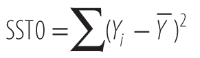
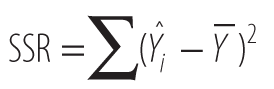
All three represent different reasons why Y values vary around their mean. Check out the diagram shown in Figure 12-6, which shows the total deviation partitioned into two components, SSR and SSE, for the first observed value.

Figure 12-6: Partitioning the Total Deviation around y.

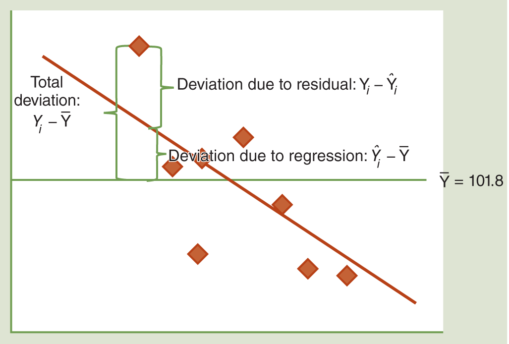
Here you can see how the total deviation of each observed Y value can be partitioned into two parts: the deviation due to the difference between the mean of Y and the regression line and the deviation between the observed value and the regression line. As it turns out, R-squared is simply the ratio of the second sum of squares over the total sum of squares.

Some variance is due to the regression itself, and some is due to error in the model. Here are the definitions of the sums of squares we’re interested in, the total sum of squares (SST0), the sum of squares due to regression (SSR), and the sum of squares due to error (SSE).

1. 
   SST0 represents the sum of the squared distance of each observed Y value from the overall mean of Y. You can see the distances that are squared and summed in Figure 12-6 under the heading “Total Deviation.”
2. 
   SSR represents the sum of the squared distance of the fitted regression line to the overall mean of Y. This is the variation that is due to the regression model itself.
3. 

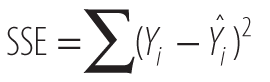
SSE represents the sum of the squared distance between the observed Y values and the regression line. This is the variation that is due to the difference between our observed values and our model, also known as the error in our model.

Let’s take a minute and calculate these values by hand for the model in our example.

To calculate SST0, subtract each observed Y from the mean of Y, and square that value like this:

SST0
IQ [Yi]		Yi -	(Yi - )2
125	101.8	23.20	538.24
109	101.8	7.20	51.84
110	101.8	8.20	67.24
117	101.8	15.20	231.04
110	101.8	8.20	67.24
98	101.8	-3.80	14.44
94	101.8	-7.80	60.84
90	101.8	-11.80	139.24
84	101.8	-17.80	316.84
81	101.8	-20.80	432.64

Now, sum the right-most column, and we get our SST0:

To calculate SSR, subtract the mean of Y from the fitted value on our regression line and square it:

SSR
Ŷ		(Ŷ - )	(Ŷ - )2
118.02	101.8	16.22	263.17
112.65	101.8	10.85	117.67
110.69	101.8	8.89	79.09
109.23	101.8	7.43	55.16
107.27	101.8	5.47	29.95
103.36	101.8	1.56	2.44
99.94	101.8	-1.86	3.45
94.08	101.8	-7.72	59.60
90.17	101.8	-11.63	135.24
72.58	101.8	-29.22	853.80

Now, sum the right-most column, and we come up with the SSR:

To calculate SSE, subtract the value of the regression line from each observed Y value and square it, like this:

SSE
IQ [Yi]	Ŷ	(Yi - Ŷi)	(Yi - Ŷi)2
125	118.02	6.98	48.69
109	112.65	-3.65	13.30
110	110.69	-0.69	0.48
117	109.23	7.77	60.42
110	107.27	2.73	7.44
98	103.36	-5.36	28.77
94	99.94	-5.94	35.32
90	94.08	-4.08	16.64
84	90.17	-6.17	38.08
81	72.58	8.42	70.89

Now, sum the column on the far right to come up with the SSE:

Now we have all the information we need in order to compute R². To do so, compute:

The section of a printout from SPSS that pertains to R-squared is shown here:

Model Summary
Model	R	R-Squared	Adjusted R-Squared	Std. Error of the Estimate
1	0.913a	0.833	0.812	6.32488
aPredictors: (Constant), BLL

So, our calculations match . . . hooray!

The standard error of the estimate tells you the average amount of error there will be in the predicted outcome (in this case, weight) using this model. (It is the standard deviation of the residuals for those statisticians among you. See the “From the Statistician” titled “What Is a Residual?” earlier in this chapter to learn more.) In this example, when using both age and height as independent variables, the weight you will predict will be off by an average of approximately 17 pounds. Obviously, you want your prediction to be as accurate as possible, so you would like to see the standard error of the estimate as close to zero as possible.

So now that you know what all of these columns mean, let’s go back to the R² of 85%, which sounds pretty good. But you know that, as with all other statistical tests, we still need to look at the p-value to see if it is significant. With multiple regression, you need to see if the R² is significant, but you also need to see if each of the independent variables is significant as well. You could have a significant R² with an independent variable that really is not adding anything to the regression model, in which case you wouldn’t want to keep that variable in your equation.

Okay, so how do we do all of this? Well, let’s take it step by step. If I ask Statistical Package for the Social Sciences (SPSS) to tell me the R-squared change, I can see what happens to the R-squared each time I add another independent variable to the regression model.

This output shows me that when I added the variable of age, the R-squared went from 0 to 0.43, and it had a p-value of 0.028, which is significant, assuming an alpha of 0.05. When I added height to the model (which now includes age and height as independent variables), the R-squared went from 0.43 to 0.85 (from explaining 43% of the variance to explaining 85% of the variance), or a change of 0.42 (42%), which had a p-value of 0.001, which is also significant at an alpha of 0.05. Adding the second independent variable increased the accuracy of predictions made with this model by increasing the amount of variance accounted for by the model.

If we look at the next table SPSS gives us, you will see an ANOVA table.

In this table you can see the p-value for both the first model (just age included) and the second (age and height included). The first model had a p-value of 0.028, and the second model had a significance level of 0.001.

The last table we see in SPSS shows us the coefficients, or the b values, in our regression equation.

When we use regression to make predictions, we should look at the column for the unstandardized coefficients (B). First, the B of 584.8 is the constant for our prediction equation. Then you will see the beta coefficients for our independent variables of age and height. This is just the b value in the regression equation. It tells us what a one-unit change in the independent variable will do to the outcome or dependent variable when the other independent variables are held constant. In this example, including both variables in the model gives us b₁ = 1.712 and b₂ = 10.372. Yikes, we are getting really statistical here—how about a little plain English?

This means that when we control for height, every additional year of age adds 1.71 pounds, and when we control for age, every additional inch of height adds 10.37 pounds. That should make sense—being taller and getting older both tend to add weight—not a pretty picture but the reality most of us face anyhow. Both age (p = 0.010) and height (p = 0.001) are significant, which means even when you control for the other, both add to the ability of the model to predict weight. If one of these variables was not significant at this point, it would indicate that when we controlled for the other variables, this variable was not significantly adding to the model or did not increase the ability of the model to make an accurate prediction.

When selecting variables to include in a model, researchers should be aware of the potential for multicollinearity concerns. Multicollinearity occurs when two or more independent variables are closely correlated. I ran into this issue in a study I completed evaluating current pregnancy desire. I asked about multiple predictor or independent variables, but two in particular were a problem: the number of previous pregnancies and the number of previous births. The two variables measure different but closely related conditions. Over 50% of my sample had the exact same value for these variables. When multicollinearity occurs, changes in one independent variable change the outcome variable, but they also change the other correlated independent variable. The two predictor variables overlap too much. Leaving them both in the model decreases the precision of the coefficient and the power associated with the regression model. But what is a researcher to do? Start by examining the correlation between the variables and calculate the variance inflation factor (VIF). Your computer program will likely produce this for you, and you just need to look for it in your output.

Here are the VIFs for CKD_Status, Wt_lbs, and Ht_inches:

A VIF of 1 means there is no correlation between the variables. A VIF between 1 and 5 indicates a moderate correlation. If the VIF is >5, you may need to consider dropping one of the correlated variables or making adjustments.

Another decision to be made has to do with how we enter variables into a regression model and what to do about any potential interactions between independent variables you want to measure and include in the model. There are whole books written on these topics, so I won’t discuss them in this chapter. Just suffice it to say, researchers shouldn’t just enter a bunch of independent variables into the computer and see which ones look significant without a rationale for why they are doing what they are doing.

In our example, the analysis gives us a regression equation we can then use to predict weight:

Weight = -584 + 1.71(years of age) + 10.37 (height in inches) + error

If a 20-year-old patient was 70 inches tall, you would predict that she might weigh

-584 + 1.71(20) + 10.37(70) = 176.1 pounds

Now I have to put in one more disclaimer here: making predictions is a highly complex process in statistics, and what we covered here is only the first step. For what you need to know at this point, I believe using the word prediction is still the best way to explain the topic, but it probably made a few statisticians twitch. Just remember, there is more to come as you go on with your statistics knowledge—such fun to look forward to!

Now there is one last form of regression that I think you should know about: logistic regression. Remember that multiple regression involves a continuous dependent variable that is at the interval or ratio level. Logistic regression is used when you have a categorical dependent variable with two categories (nominal or ordinal with two categories), such as living or dying. (Multinomial logistic regression can be used when the dependent variable has more than two categories, but it is beyond the scope of this text—whew!) One of the advantages of using logistic regression is that the technique generates an odds ratio (OR), which is the odds or probability of the outcome occurring divided by the odds or probability of the outcome not occurring.

From the Statistician

Brendan Heavey

Methods: Multiple Regression

To tell you the truth, learning how to estimate parameters in a multiple regression model is not worth the time it would take to learn unless you have a little background in linear algebra. If you happen to have a good sense of working with matrices, I would encourage you to take a full course in regression because most of the fundamentals are exceptionally interesting. In this text, however, we’re going to assume that the way you will estimate parameters in regression models with multiple independent variables is by setting up the model in a statistical computing package like SPSS and making the computer perform the calculations for you.

Let’s say, for instance, we are interested in expanding our study of the effect that BLL has on children’s IQ. A second variable that we may have some interest in is the IQ of each child’s mother. Because of this interest, we might include another question in the study’s survey and have data that look like this:

BLL (mcg/dL)	Mother’s IQ	Child’s IQ
7	120	125
18	111	109
22	119	110
25	115	117
29	110	110
37	100	98
44	125	94
56	80	90
64	81	84
100	95	81

In this case, we have two independent variables, BLL and mother’s IQ, and we’re interested to see how well we can determine what a child’s IQ will be given both of these predictors. So, in essence, we want to set up a multiple regression model in SPSS with two independent variables, BLL and mother’s IQ, and one dependent variable, child’s IQ.

There are two differences in the setup of this model from the one we set up in the last “From the Statistician” feature. First, your data set will have another variable, so it will look like this:

Reprint Courtesy of International Business Machines Corporation, © International Business Machines Corporation. SPSS Inc. was acquired by IBM in October 2009. IBM®, the IBM logo, ibm.com, and SPSS® are trademarks or registered trademarks of International Business Machines Corporation, registered in many jurisdictions worldwide. Other product and service names might be trademarks of IBM or other companies. A current list of IBM trademarks is available on the Web at “IBM Copyright and trademark information” at www.ibm.com/legal/copytrade.shtml.

Next, when you set up the regression, you will have to add a second variable, MothersIQ, to the list of independent variables, like this:

Reprint Courtesy of International Business Machines Corporation, © International Business Machines Corporation. SPSS Inc. was acquired by IBM in October 2009. IBM, the IBM logo, ibm.com, and SPSS are trademarks or registered trademarks of International Business Machines Corporation, registered in many jurisdictions worldwide. Other product and service names might be trademarks of IBM or other companies. A current list of IBM trademarks is available on the Web at “IBM Copyright and trademark information” at www.ibm.com/legal/copytrade.shtml.

The resulting tables will have almost the exact same structure as before but with different data. The only really big difference in the design of the resulting table is that there will now be three parameters in the “Coefficients” table, which is reproduced here:

Coefficientsa
Model	Unstandardized Coefficients		Standardized Coefficients
	B	Std. Error	Beta	t	Sig.
1 (Constant) BLL Mother’s IQ	99.624 -0.420 0.180	21.261 0.102 0.173	-0.784 0.198	4.686 -4.132 1.042	0.002 0.004 0.332
aDependent variable: IQ.

Notice that there are three parameters: the y-intercept or constant, BLL level, and mother’s IQ. Each parameter has a coefficient, which is equivalent to what we would call the slope if this were a functional relationship. Therefore, this model can be written as:

Y= -0.419556X₁ + 0.180322X₂ + 99.624035 + ε

Note: By default, SPSS shows parameter estimates to three decimal places, but for this example, we have performed some magic to get the estimates out to a few more decimals so that the results all tie together.

And you can think of this model as:

IQ = -0.419556 BLL + 0.180322 × Mother’s IQ + 99.642035 + Error

So now, if we’re interested in what IQ level this model would result in based on a child with a BLL of 7 mcg/dL and a mother’s IQ of 120, we would plug these two Xs into the regression equation and come up with the following result:

Based on the same logic, we would come up with the following fitted values for our regression function (in the right-most column):

X1 BLL (mcg/dL)	X2 Mother’s IQ	IQ
7	120	125	118.33
18	111	109	112.09
22	119	110	111.85
25	115	117	109.87
29	110	110	107.29
37	100	98	102.13
44	125	94	103.70
56	80	90	90.55
64	81	84	87.38
100	95	81	74.80

Now, something really interesting: once you calculate all of the Ŷs, the rest of the model equations are exactly the same as in the single predictor case:

Here are all the numbers we’ll need to calculate SST0:

Yi		(Yi - )2	(Yi - )2
125	101.8	23.2	538.24
109	101.8	7.2	51.84
110	101.8	8.2	67.24
117	101.8	15.2	231.04
110	101.8	8.2	67.24
98	101.8	-3.8	14.44
94	101.8	-7.8	60.84
90	101.8	-11.8	139.24
84	101.8	-17.8	316.84
81	101.8	-20.8	432.64

Now, sum the right-most column:

SSTO = 1919.6

Next, SSR’s formula:

And all the data we’ll need:

Ŷi		(Ŷi - )	(Ŷi - )2
118.33	101.8	16.53	273.11
112.09	101.8	10.29	105.84
111.85	101.8	10.05	101.05
109.87	101.8	8.07	65.16
107.29	101.8	5.49	30.17
102.13	101.8	0.33	0.11
103.70	101.8	1.90	3.63
90.55	101.8	-11.25	126.46
87.38	101.8	-14.42	207.98
74.80	101.8	-27.00	729.05

Sum the right-most column:

SSR = 1642.535

SSE’s formula is:

All the data:

Yi	Ŷi	(Ŷi - )	(Yi - Ŷi)2
125	118.33	6.67	44.54
109	112.09	-3.09	9.54
110	111.85	-1.85	3.43
117	109.87	7.13	50.80
110	107.29	2.71	7.33
98	102.13	-4.13	17.08
94	103.70	-9.70	94.17
90	90.55	-0.55	0.31
84	87.38	-3.38	11.42
81	74.80	6.20	38.45

Sum the right-most column:

SSE = 277.065

Which is great because that’s what the output from SPSS tells us in the ANOVA table for this model:

ANOVAa
Model	Sum of Squares	df	Mean Square	F	Sig.
1 Regression	1642.535	2	821.268	20.749	0.001b
Residual	277.065	7	39.581
Total	1919.600	9
aDependent variable: IQ. bPredictors: (Constant), mother’s IQ, BLL.

Now, let’s examine the resulting R². We could calculate it ourselves using the same equation as before, substituting the values in the ANOVA table for SST0 and SSR:

Or we could just look at the first table produced by the computer program for this model:

Model Summary
Model	R	R-Squared	Adjusted R-Squared	Std. Error of the Estimate
1	0.925a	0.856	0.814	6.29132
aPredictors: (Constant), mother’s IQ, BLL.

Finally, let’s look back at the R² value from the model with one predictor variable:

Model Summary
Model	R	R-Squared	Adjusted R-Squared	Std. Error of the Estimate
1	0.913a	0.833	0.812	6.32488
aPredictors: (Constant), BLL.

Notice that our R² went from 0.833 to 0.856 just by adding a second predictor. An R² that results from a model with multiple independent variables will always be greater than or equal to the R² from any of the models resulting from fewer of these same independent variables. Said a different way, when adding more and more predictors, R² will never go down.

Regression analysis is a statistical procedure that allows us to develop a regression equation that we can use to infer or predict future events. There are several types of regression. In this chapter, we discussed linear regression, multiple regression, and logistic regression. Linear regression analyzes the relationship between a single independent variable and a single interval- or ratio-level dependent variable. The slope (b) of the linear regression equation tells us how much the predicted value of the dependent variable changes when there is a one-unit change in the independent variable. The residual is the prediction error, or how far away the actual data points fall from the prediction line.

When researchers want to predict how two or more variables affect a dependent variable, they may use multiple regression, where the values of the regression coefficients (b) show the change in the dependent variable for a one-unit increase in the independent variable with which it is associated. Each regression model has a corresponding R-squared, which tells you how much of the variance in the dependent variable (outcome) is explained by the independent variables you have included in the model or equation. When the sample size is small, researchers sometimes report the adjusted R-squared to avoid overestimating the amount of variance in the dependent variable explained by the independent variables in the equation. The R-squared change tells you the additional variance in the dependent variable when you add another independent variable. Make sure the R-squared change is statistically significant if you want to increase the accuracy of your prediction equation.

There will always be some error involved in any prediction (yes—even yours!), and with multiple regression, we see this estimated by the standard error of the estimate. Researchers try to make the standard error of the estimate as small as possible, obviously trying to make their predictions as accurate as possible.

The final form of regression we discussed was logistic regression, which we use when the outcome or dependent variable is binary, such as for mortality. Logistic regression lets researchers report an odds ratio that tells them the odds or probability of the outcome event occurring in one group versus another.

Questions 1-4: Mosfeldt et al. (2012) collected data on 792 patients age 60 or over who were admitted to a hospital in Denmark with a hip fracture between 2008 and 2010. They reported that an elevated creatinine level upon hospital admission for a hip fracture (>90 mmol/L for women and >105 mmol/L for men) is associated with an almost threefold increase in mortality risk.

1. What is the independent variable? At what level of measurement is it?

   Show Answer

2. What is the dependent variable? At what level of measurement is it?
3. What type of sample is this? Is it a probability or nonprobability sample?

   Show Answer

4. These researchers chose to use a regression model. Should they perform a linear regression, multiple regression, or logistic regression? Why?

5. What would be the independent variables? At what level are these variables?

   Show Answer

6. What would be the dependent variable? At what level is it?
7. What type of sampling method is this? Is it probability or nonprobability sampling?

   Show Answer

8. Why might these researchers have chosen to exclude those admitted with a hip fracture who are younger than 60?
9. Would it be appropriate to use these results to predict the length of stay for female patients over age 60 admitted with hip fractures? Why or why not?

   Show Answer

10. If these researchers had already established that a causative relationship existed between these variables and asked you for a statistics consultation, what would you tell them is the appropriate regression technique to apply? Explain your answer.

11. According to the SPSS output, what percentage of the variance in health knowledge is explained by age and academic knowledge?

    Show Answer

12. Is the R-squared significant? Explain your answer.
13. Should the nurse researcher include both independent variables in her final model? Explain your answer.

    Show Answer

14. If the nurse researcher includes both independent variables in her prediction equation, her predicted health knowledge score will be incorrect by an average of how many points?
15. According to this model, every 1-year increase in age results in what change in the health knowledge score?

    Show Answer

16. Using this model, if a 15-year-old scored 70 on his academic knowledge exam, what would you expect him to score on his health knowledge exam?
17. What type of sample is this?

    Show Answer

18. A researcher working with military officers would like to use the data he has collected from them to predict their health knowledge score based on this research. Would this be an appropriate application of this prediction equation? Why or why not?

19. Does this model explain more or less of the variance in the health knowledge score? Is this a large change? Does that make sense?

    Show Answer

20. In which model is the predicted outcome more accurate?
21. Using this prediction equation, if a 15-year-old scored 70 on his academic knowledge exam, what would you predict he would score on his health knowledge exam?

    Show Answer

22. Show this frequency distribution graphically.
23. At what level of measurement is age in this example?

    Show Answer

24. Calculate all appropriate measures of central tendency for this variable.
25. Is age normally distributed in this sample? Explain your answer.HbA1c = 0.387 (FBS) + 4.855

    Show Answer

26. From this equation, you know that a one-unit increase in FBS is associated with what change in HbA1c?
27. The researchers also examined the independent variable of gender but did not include this variable in the final regression equation. Why do you think gender was not included in the final regression model?

    Show Answer

28. The researchers report that ethnicity was not measured in this study but has been reported to be significant in other similar studies. If the study was repeated with ethnicity included, and if none of the independent variables was then significant, we would know the original study that reported FBS was significantly related to HbA1c had made what type of error?FBS = 1.33(HbA1c) - 2.528

29. If HbA1c is 8%, what would be the predicted value, in mmol/L, of FBS?

    Show Answer

30. If HbA1c increases by 2%, what would be the predicted change in FBS?Weight = 50 + 2 (height in inches) + 2.4 (gender) - 3.1 (age)

31. How does being under age 40 affect weight?

    Show Answer

32. According to this study, an individual who is 66 inches tall, not male, and age 49 would weigh how much?
33. How would the predicted weight change with a 1-inch increase in height?

    Show Answer

34. The R² value of this model is 0.64. You know this means:
35. You also collected data on hours of daily activity. When you introduce this variable into the model, the R² becomes .66, and the R² change has p = 0.18. Would you recommend keeping the variable?

    Show Answer

36. You also collected data on waist circumference. When you checked the variance inflation factor for waist circumference and height, you found a strong correlation. Should you include waist circumference as an independent variable?

Research Application Article

Because regression is a complex statistical technique, you will see that most articles that use it can be a little more challenging to sort through. They also often use a variety of other statistical techniques we did not cover in this course. So be patient with yourself. Take your time working through the following article review, and you may surprise yourself with how much you do understand and can interpret with the knowledge you learned in this chapter.

Poghosyan, L., Ghaffari, A., Liu, J., and McHugh, M. D. (2020). Organizational support for nurse practitioners in primary care and workforce outcomes. Nursing Research, 69(4), 280-288. https://doi.org/10.1097/NNR.0000000000000425

1. What was the purpose of this article?

   Show Answer

2. When is it appropriate to use logistic regression, and when was it used in this study?
3. The study included organizational support and resources (OSR) variables along with nurse practitioner (NP) age, gender, race, number of years in current position, work hours in the past week, practice type, number of NPs in the practice, and if the NP managed a panel of patients. The inclusion of these independent variables allows for the impact of these variables to be controlled and the impact of the OSR variables to be isolated and examined specifically. Why did the researchers test for multicollinearity among the independent variables?

   Show Answer

4. What was the size of the sample, and where was it collected?
5. Identify at least one characteristic of the sample that limits the generalizability of the study.

   Show Answer

6. The researchers completed their analyses using both an individual OSR score and an organizational level OSR (mean of all the OSR scores from the NPs in the practice). They assessed the internal consistency of both OSR scales using Cronbach’s alpha. Look at Table 2 in the article. Which item on the individual OSR had the lowest Cronbach’s alpha level? Was it higher or lower than the Cronbach’s alpha for the organizational OSR? What does that mean?
7. Look at the results for the organizational-level OSR and intent to leave current job. In this regression model, there is an OR of 0.29, which means that every one-unit increase in the organizational OSR results in a 71% (1 - .29 × 100) decrease in the odds of intent to leave. Is this result significant?

   Show Answer

8. Look at the results for the organizational-level OSR and quality of care. What is the value of the regression coefficient, and what does this mean in plain English?
9. Look at Table 5 in the article. The intent-to-leave analysis has ORs listed for the various independent variables in the regression equation. What is the OR for the relationship between an organizational OSR score of “Good” and intent to leave? Describe this relationship.

   Show Answer

10. Look at Table 5 in the article. The intent-to-leave analysis has ORs listed for the various independent variables in the regression model. What is the OR for the relationship between NPs NOT having their own panel of patients and intent to leave? Describe this relationship.
11. A federally funded health center in your state has a very high turnover rate for NPs. How might the results from this article affect the recommendations you might make?

    Show Answer

1. Creatinine level, interval/ratio

3. Convenience, nonprobability

5. Creatinine levels upon admission and hemoglobin levels upon admission, interval/ratio level

7. Cluster sampling, probability sampling

9. No, the sample includes only men, so it is not representative of a population of women.

11. R-squared = 74.7%, adjusted R-squared = 74.3%

13. No, the beta for age is 2.711, with a significant p-value (p = 0.000), whereas the b for academic knowledge is -0.023, which is insignificant (p = 0.43).

15. An increase of 2.711 points (unstandardized age coefficient = 2.711)

17. Random or probability sample

19. The model explains slightly less of the variance in the health knowledge score. (R-squared changes from 0.747 to 0.746.) This is not a large change, which makes sense because an independent variable was eliminated in this model, but it was an insignificant independent variable, so the change should be small.

21. 81.08 = 39.89 + 2.746(15)

23. Interval

25. No, the mean, median, and mode are not equal; therefore, we know the sample is not normally distributed.

27. Gender was not a significant independent variable and was not included to minimize the prediction error.

29. 1.33(8) - 2.528 = 8.112

31. Being under age 40 decreases the weight prediction by 3.1 pounds.

33. Increase of 2 pounds

35. No, the p-value of the R² change is greater than 0.05.

Answers to Research Application Article Questions

1. To look at how the various facets of OSR affect (a) job satisfaction, (b) intent to leave, and (c) quality of care.

3. Because if there is significant overlap between what the variables measure, then the independent variables are no longer independent from each other, and changes in one affect the other correlated independent variable plus the dependent variable. This decreases the precision of the coefficients and decreases the power of the regression model.

5. Limiting factor answers may vary. (a) The database only has information from NPs employed in practices with physicians; thus, no NPs from nurse-managed clinics without MDs are included. (b) All NPs were practicing in one state. (c) Almost all of the respondents were white and female. (d) Convenience sampling was utilized, which is a nonprobability sampling method.

7. Yes. (a) p< 0.5, which means it is significant at an alpha level of 0.05.

9. OR = 0.17, which is significant. This means having a good organizational OSR score was protective from having the intent to leave the job. Those with a good OSR score had a significantly lower probability of intending to leave their jobs than those who had poor OSR scores.

11. Answers will vary but may include the following: Providing organizational support to NPs is associated with higher job satisfaction, less intent to change positions, and improvements in quality of care. The board of directors may wish to work with the practice managers to consider how organizational support, such as the availability of personnel support, task assistance, resources for patient care time, and access to information, is being handled within the clinic.