Nonparametric Tests

The principal goal of this chapter is help you understand the use of nonparametric tests for group comparisons when the assumptions of parametric tests are violated. This chapter will prepare you to:

Distinguish between parametric tests and nonparametric tests.

Evaluate assumptions of nonparametric tests of differences.

Distinguish between independent sample difference tests and dependent sample difference tests.

Distinguish between two samples and more than two samples difference tests.

Report the findings correctly in APA style.

Understand the application of nonparametric tests in evidence-based practice.

Wilcoxon rank-sum test

Wilcoxon signed-rank test

Up to this point, we have discussed different types of parametric tests, such as the independent samples t-test and variations of analysis of variance (ANOVA). Parametric tests have a set of assumptions that usually include a distributional assumption such as normality. For accurate statistical results, we need to ensure that assumptions are met before the analysis. Investigators may use a parametric test even when one or more violations of the assumptions are present as long as the violations are not serious. However, there are occasions where serious violations of these assumptions occur, and such violations negatively influence the internal and external validity of a study’s findings. Nurse investigators often find ourselves conducting studies that will have a nonnormal distribution; for example, when we conduct pilot studies with small samples, or when we must rely on a convenience sample. Thankfully, nonparametric tests provide statistical solutions for such situations.

CASE STUDY

Data from Connors, J. T., Hodges, E. A., D’Auria, J., & Windham, L. (2018). Implementing vaccine hesitancy screening for targeted education. Journal of the American Association of Nurse Practitioners, 30(8), 450μ459.

According to the Centers for Disease Control and Prevention (CDC), lower vaccination rates among children have contributed to the resurgence of preventable infectious diseases. A key issue related to unvaccinated children seems to be the hesitancy of parents to vaccinate their children. Connors, Hodges, D’Auria, and Windham (2018) reported the results of a study designed to identify if use of a vaccine hesitancy tool with a provider discussion affected parental decisions to vaccinate. The researchers conducted a descriptive study using a convenience sample with parents of children 2 months to 6 years of age presenting for a well-child visit at a pediatric clinic. They measured the difference between parents’ responses to questions on the vaccine hesitancy tool previsit and postvisit.

Of interest here, the authors use the Wilcoxon signed-rank test to evaluate the differences between the previsit and postvisit responses. Why use this test in this particular situation? In this study, measurements were at the ordinal level, we cannot assume a normal distribution, and a nonparametric statistical test is appropriate.

Results indicated that there was a substantial statistical difference (p = .033, z = 0.724) only in the category of “trust” out of the vaccine hesitancy categories of trust, efficacy beliefs, safety concerns, prevalence beliefs, and vaccination beliefs. The investigators concluded that the change in trust was a result of participants selecting different positive responses to the provider discussion on vaccines, but a larger study with a more diverse sample is needed before the findings are generalizable.

When data are not normally distributed, we can use nonparametric tests (tests that do not rely on a distributional assumption). Most nonparametric tests analyze the rank of the data, not the actual raw data. When assumptions of normality are met, parametric tests tend to be more powerful than nonparametric tests. However, nonparametric tests become more powerful in finding an effect when distributional assumptions are violated. Nonparametric tests serve the same purposes as their parametric counterparts, but they allow us to take a more conservative approach to analysis when some aspect of the test assumptions is violated.

When making group comparisons when the distributional assumption of the independent samples t-test is violated, the nonparametric counterparts, the Wilcoxon rank-sum test and the MannμWhitney test, should be used. Let us consider an example where we compare family satisfaction with dementia care between a traditional caregiver group (N = 13) and a music therapy group (N = 9). We know that because these sample sizes are small the distribution will not be normal; therefore, either the Wilcoxon rank-sum test or the MannμWhitney test will be appropriate for this situation instead of the independent samples t-test. The data are shown in Table 13-1.

Table 13-1 Data for Dementia Care Example: Family Satisfaction and the scale (0-30)

Traditional Caregiver Group	Music Therapy Group
1	21
12	25
17	29
15	27
9	9
15	15
17	27
19	19
13	16
7
16
3
14

Note: numbers represents Family Satisfaction and the scale (0-30)

Assumptions

As these are nonparametric tests, there are no distributional assumptions. However, these tests do assume the following:

Random sample

Two groups are independent of each other

Level of measurements is at least ordinal

Doing and Interpreting Wilcoxon Rank-Sum Test and/or MannμWhitney Test

First, we need to set up hypotheses; these are similar to those of an independent samples t-test:

H₀: The distributional functions are identical for two groups.

H_a: The distributional functions are not identical for two groups.

The test statistics for both tests are calculated using ranks of the data. When the group sample sizes are equal, the test statistic is the summed rank value that is the smallest. However, it will be the summed rank value of the group with the smaller sample size if the group sample sizes are not equal. For our example, the sum of rank value in the traditional caregiver group is 109.50, and that in the music therapy group is 143.50. Because of the unequal sample sizes, our test statistic is the summed rank value for the music therapy group, as it is the smaller sample.

Once the statistic is computed, the associated p-value is evaluated, and we make the decision to reject or not reject the null hypothesis (i.e., reject the null hypothesis when the p-value associated with the computed statistic is small, or not reject when the p-value associated with the computed statistic is large).

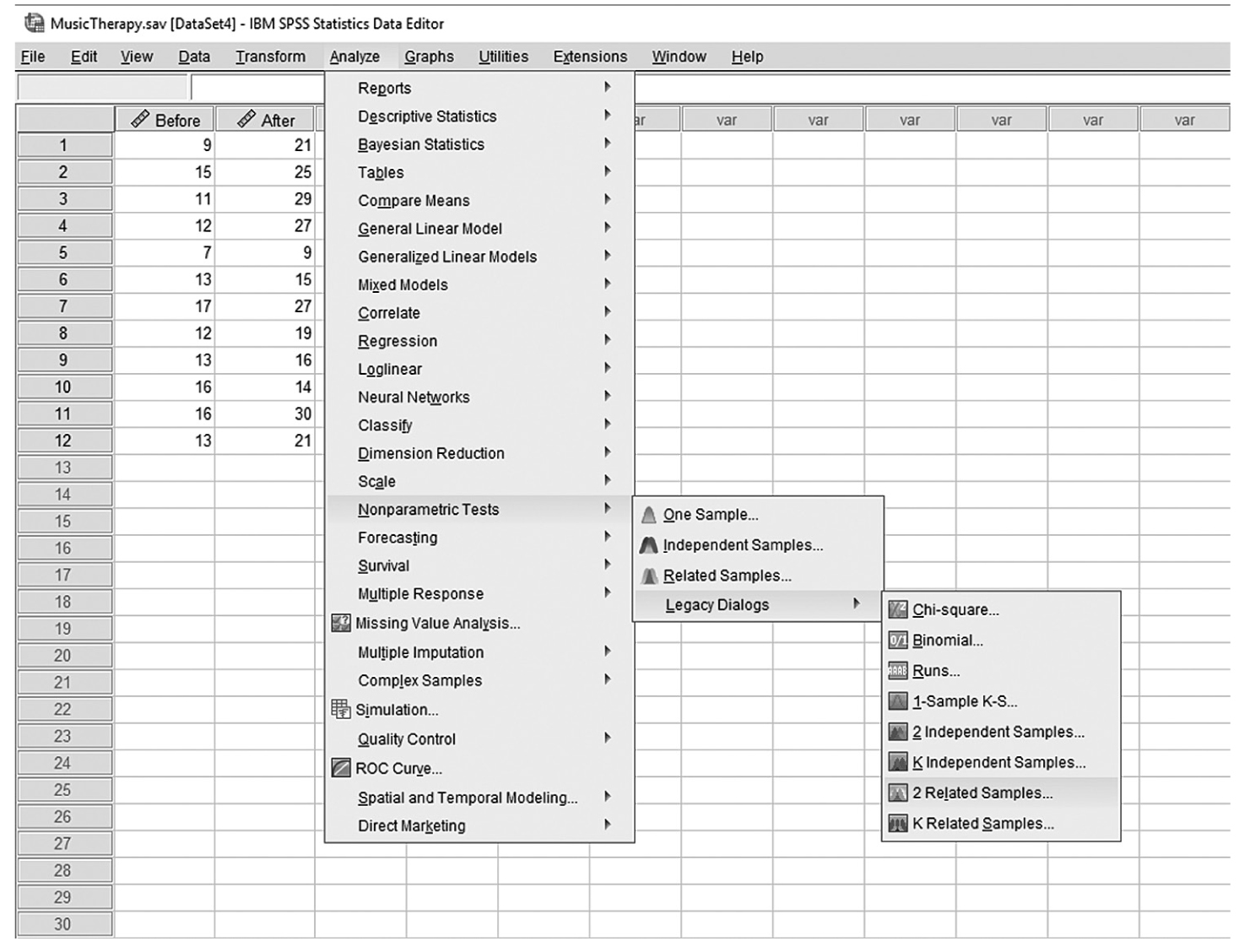
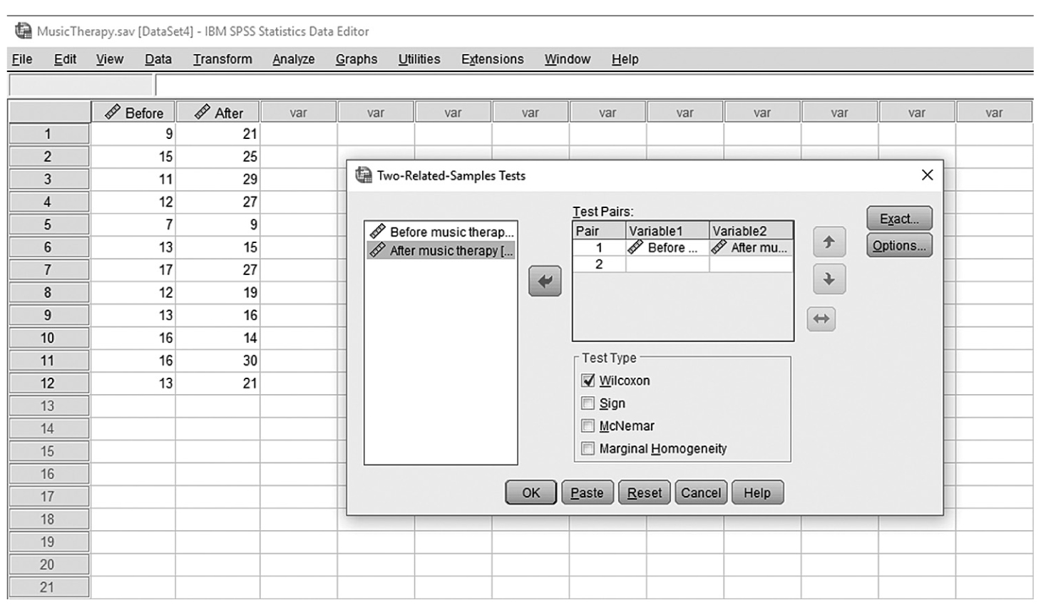
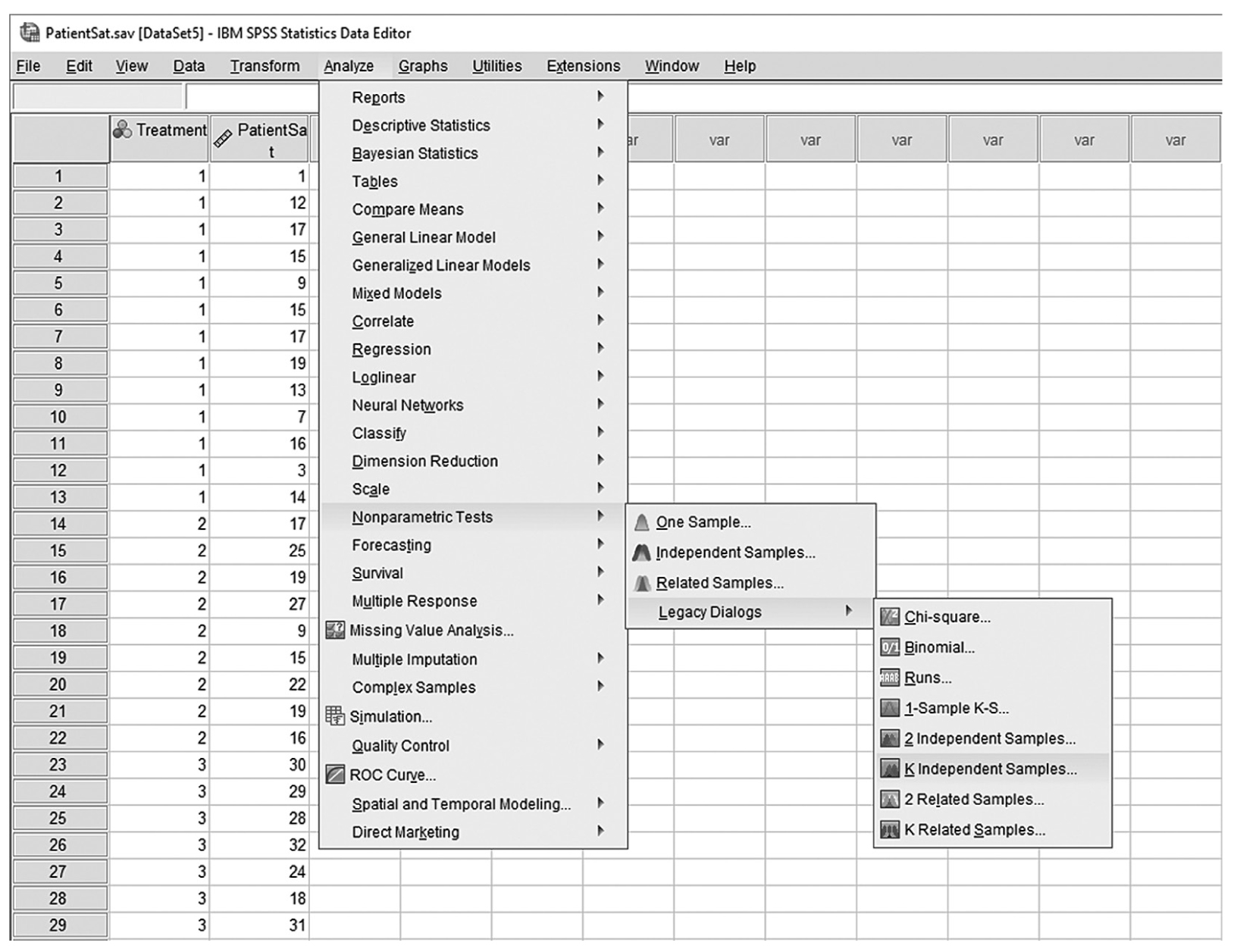
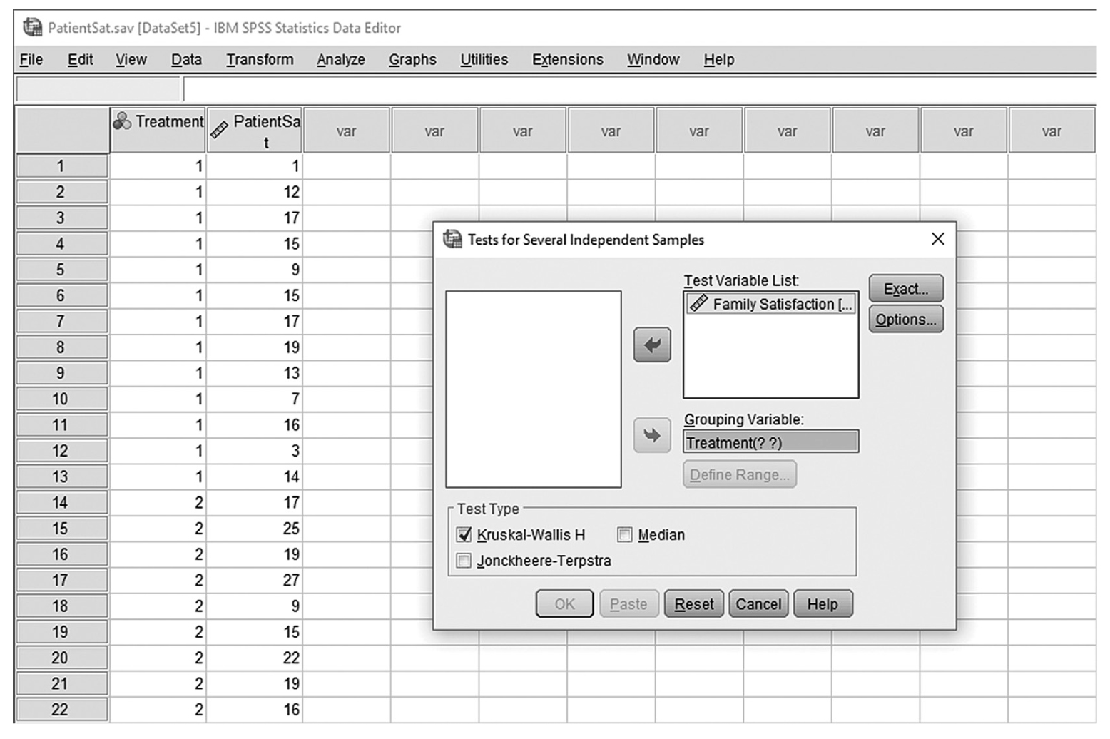
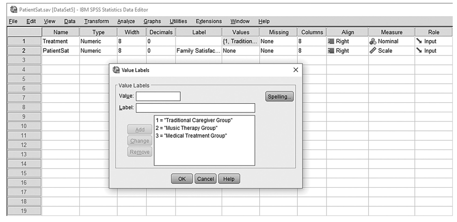
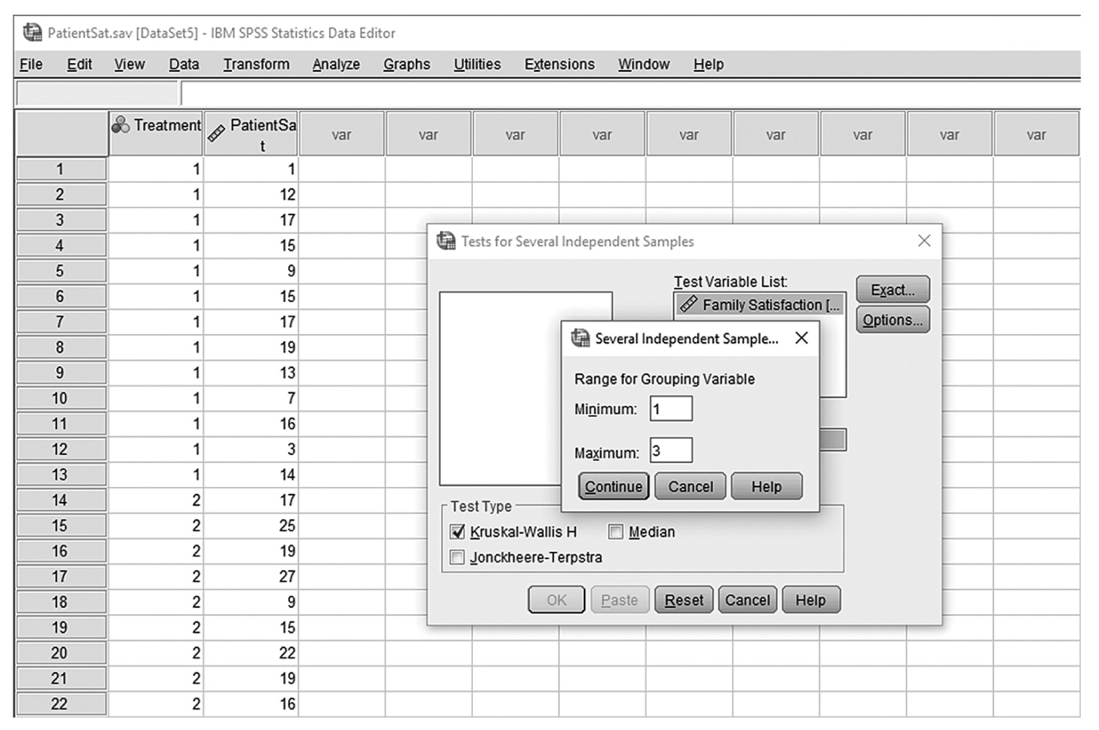
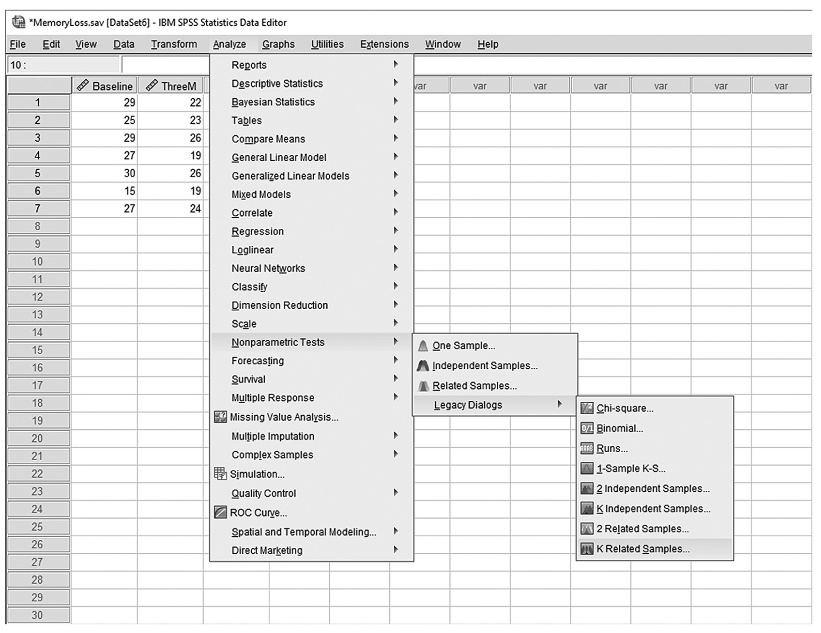
To conduct Wilcoxon rank-sum tests and/or MannμWhitney tests in IBM SPSS Statistics software (SPSS), you will open FamilySat.sav and go to Analyze > Nonparametric Tests > Legacy Dialogs > 2 Independent Samples, as shown in Figure 13-1. In the Two Independent Samples Tests dialog box, move the dependent variable, family satisfaction (“FamilySat”), into “Test Variable List,” and the independent variable, “Treatment,” into “Grouping Variable” by clicking the corresponding arrow buttons in the middle (Figure 13-2). You will notice that “MannμWhitney U” is checked by default under “Test Type”; this option will produce statistics of both Wilcoxon rank-sum tests and MannμWhitney tests. You will also notice that the “OK” button is not active because we have not yet defined our two groups. As you see in Figure 13-3, we have defined the coding of 1 for the traditional caregiver group and 2 for the music therapy group. Now click on the “Define Groups” button and assign 1 for group 1 and 2 for group 2, as in Figure 13-4. Clicking “Continue” and then “OK” will produce the output. The example output is shown in Table 13-2.

Selecting MannμWhitney tests in SPSS.

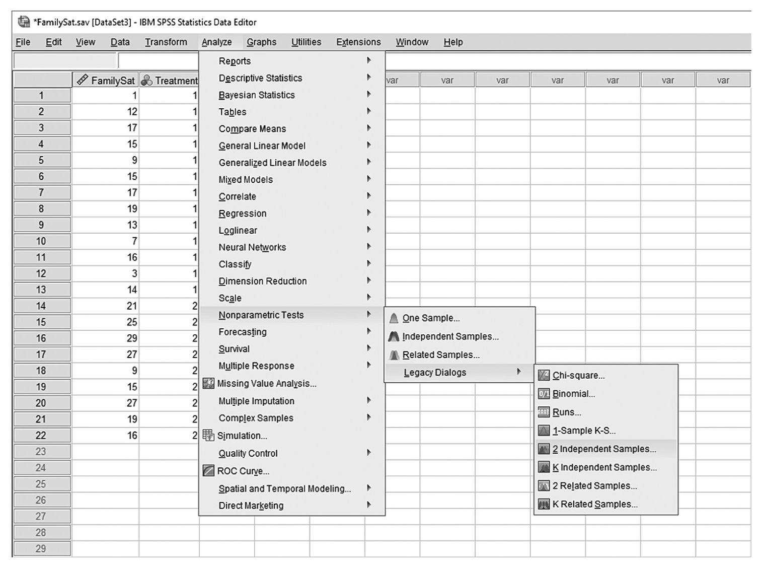
A screenshot in S P S S shows selection of the Analyze menu, with Nonparametric tests command chosen, from which Legacy Dialogs is selected, under which 2 Independent Samples option is selected. Data in the worksheet shows columns of numerical data.

Reprint Courtesy of International Business Machines Corporation, © International Business Machines Corporation. “IBM SPSS Statistics software (“SPSS”)”. IBM^®, the IBM logo, ibm.com, and SPSS are trademarks or registered trademarks of International Business Machines Corporation.

Defining variables in MannμWhitney tests in SPSS.

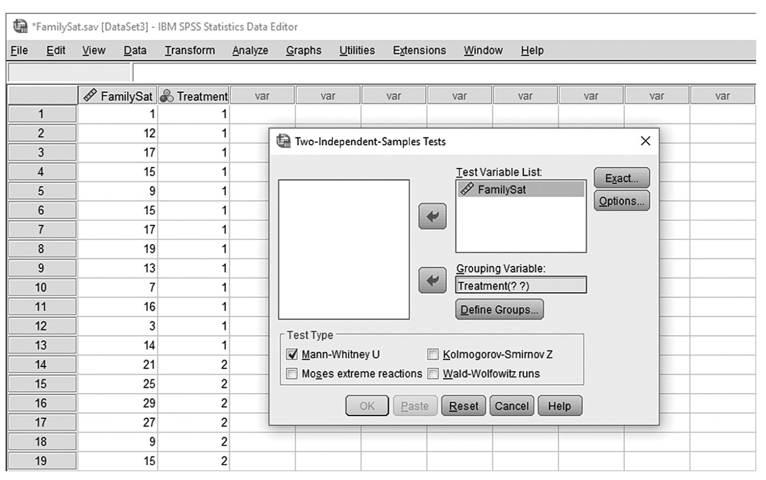
A screenshot in S P S S Editor defines variables in MannμWhitney Tests. The data in the worksheet shows columns of numerical data.

Reprint Courtesy of International Business Machines Corporation, © International Business Machines Corporation. “IBM SPSS Statistics software (“SPSS”)”. IBM^®, the IBM logo, ibm.com, and SPSS are trademarks or registered trademarks of International Business Machines Corporation.

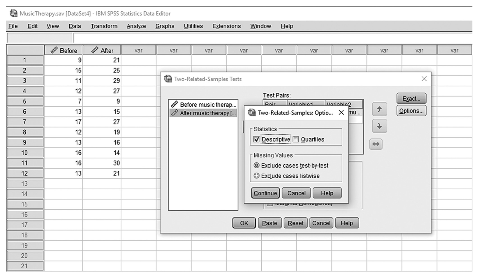
Coding scheme for the “Treatment” variable.

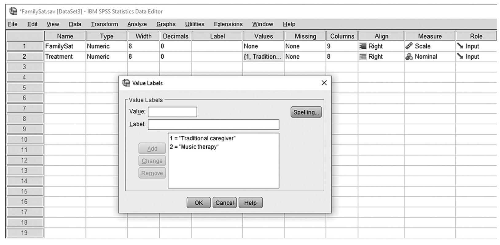
A screenshot in S P S S depicts the coding scheme for the variable, Treatment.

Reprint Courtesy of International Business Machines Corporation, © International Business Machines Corporation. “IBM SPSS Statistics software (“SPSS”)”. IBM^®, the IBM logo, ibm.com, and SPSS are trademarks or registered trademarks of International Business Machines Corporation.

Defining groups in MannμWhitney tests in SPSS.

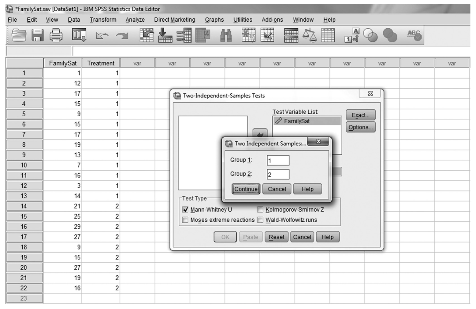
A screenshot in S P S S shows a dialog box, where groups are defined in a two-independent samples t-test. There are two columns, FamilySat and Treatment, with rows of numerical data under each column.

Reprint Courtesy of International Business Machines Corporation, © International Business Machines Corporation. “IBM SPSS Statistics software (“SPSS”)”. IBM^®, the IBM logo, ibm.com, and SPSS are trademarks or registered trademarks of International Business Machines Corporation.

Table 13-2 Example Output of MannμWhitney Tests in SPSS

Ranks
Treatment		N	Mean Rank	Sum of Ranks
FamilySat	Traditional caregiver	13	8.42	109.50
	Music therapy	9	15.94	143.50
	Total	22

Test Statistics^b
	FamilySat
MannμWhitney U	18.500
Wilcoxon W	109.500
Z	μ2.678
Asymp. sig. (two-tailed)	.007
Exact sig. [2 × (one-tailed sig.)]	.006^a

^aNot corrected for ties

^bGrouping variable: treatment

Reporting MannμWhitney Tests

When reporting MannμWhitney test results, you should report the size of the corresponding statistics and associated p-value as well as medians of groups, so that the readers will know how the sample statistics are different. Effect size, r, can be computed and reported with the following equation:

where Z is one of the statistics that SPSS calculates for MannμWhitney tests and N is the total number of observations. The following are examples of how to report the test results.

For MannμWhitney tests: Family satisfaction levels in the traditional caregiver group (Mdn = 14.00) did differ substantially from the music therapy group (Mdn = 21.00), U = 18.50, z = -2.68, p = .007, r =-.57.

For Wilcoxon rank-sum tests: Family satisfaction levels in the traditional caregiver group (Mdn = 14.00) differed substantially from the music therapy group (Mdn = 21.00), W_s = 109.50, z = -2.68, p = .007, r = -.57.

With a p-value of .007, we can see that family satisfaction differs substantially depending upon the type of treatment, and the group who received music therapy had substantially higher satisfaction than the group who received traditional care based on the descriptive statistics. Note that the median is and should be reported as a better measure of central tendency for nonparametric tests with no distributional assumption. You may compute the median as discussed in Chapter 6.

When the distributional assumption of dependent samples t-test is violated, the counterpart of the dependent samples t-test, the Wilcoxon signed-rank test, should be used. Consider a comparison between the amount of memory loss before (N = 12) and after (N = 12) music therapy in the same participants. We know that these sample sizes are small and the distribution will not be normal; therefore, the Wilcoxon signed-rank test should be used instead of the dependent samples t-test. The data are shown in Table 13-3.

Table 13-3 Data for Music Therapy Example

Before	After
9	21
15	25
11	29
12	27
7	9
13	15
17	27
12	19
13	16
16	14
16	30
13	21

Note: number represents amount of memory loss.

Assumptions

As the Wilcoxon signed-rank test is the nonparametric counterpart of the dependent samples t-test, it does not have distributional assumptions. However, this test does assume the following:

The sample is a random sample from a respective population.

The level of measurement of dependent variable should be at least ordinal.

Doing and Interpreting Wilcoxon Signed-Rank Tests

First, we need to set up hypotheses; these are similar to those for the dependent samples t-test:

H₀: The median difference between pairs of observations is equal to zero.

H_a: The median difference between pairs of observations is not equal to zero.

The test statistic is calculated using ranks of the data, but the signs of the difference between measurements are assigned to the corresponding rank with Wilcoxon signed-rank tests. The statistic is simply the sum of positive ranks of the difference between measurements, but the value of z in the SPSS output can be reported instead.

Once the statistic is computed, the associated p-value is then compared with alpha, and we decide to reject or not reject the null hypothesis based on the relative size of the p-value.

To conduct a Wilcoxon signed-rank test in SPSS, you will open MusicTherapy.sav and go to Analyze > Nonparametric Tests > Legacy Dialogs > 2 Related Samples, as shown in Figure 13-5. In the Two-Related-Samples Tests dialog box, you will move the variables to be paired into “Test Pairs” in order by clicking corresponding arrow buttons in the middle, as shown in Figure 13-6. You will notice that “Wilcoxon” is checked by default under “Test Type,” and this option will produce statistics of Wilcoxon signed-rank tests. Clicking “Continue” and then “OK” will then produce the output. Notice that you can request descriptive statistics by clicking on the “Options” button and checking “Descriptive” in the Two Related Samples dialogue box, as shown in Figure 13-7. The example output is shown in Table 13-4.

Selecting Wilcoxon signed-rank tests in SPSS.

A screenshot in S P S S shows the selection of the Analyze menu, with Nonparametric tests command chosen, from which Legacy Dialogs is selected, under which Two-related samples option is selected. Data in the worksheet shows columns of numerical data.

Reprint Courtesy of International Business Machines Corporation, © International Business Machines Corporation. “IBM SPSS Statistics software (“SPSS”)”. IBM^®, the IBM logo, ibm.com, and SPSS are trademarks or registered trademarks of International Business Machines Corporation.

Defining variables in Wilcoxon signed-rank tests in SPSS.

A screenshot in S P S S shows a dialog box, with heading Two-related samples tests. Data in the worksheet shows columns of numerical data.

Reprint Courtesy of International Business Machines Corporation, © International Business Machines Corporation. “IBM SPSS Statistics software (“SPSS”)”. IBM^®, the IBM logo, ibm.com, and SPSS are trademarks or registered trademarks of International Business Machines Corporation.

Requesting descriptives for Wilcoxon signed-rank tests in SPSS.

A screenshot in S P S S shows a dialog box, where groups are defined in a two-related samples t-test. There are two columns, Before and After, with rows of numerical data under each column.

Reprint Courtesy of International Business Machines Corporation, © International Business Machines Corporation. “IBM SPSS Statistics software (“SPSS”)”. IBM^®, the IBM logo, ibm.com, and SPSS are trademarks or registered trademarks of International Business Machines Corporation.

Table 13-4 Example Output of Wilcoxon Signed-Rank Tests in SPSS

Ranks
		N	Mean Rank	Sum of Ranks
After music therapyμbefore music therapy	Negative ranks	1^a	2.00	2.00
	Positive ranks	11^b	6.91	76.00
	Ties	0^c
	Total	12

^aAfter music therapy before music therapy.

^bAfter music therapy > before music therapy.

^cAfter music therapy = before music therapy.

Test Statistics^b
	After Music TherapyμBefore Music Therapy
Z	μ2.908^a
Asymp. sig. (two-tailed)	.004

^aBased on negative ranks

^bWilcoxon signed-rank test

Reporting Wilcoxon Signed-Rank Tests

When reporting Wilcoxon signed-rank test results, you should report the size of corresponding statistics and the associated p-value; also, be sure to report medians of repeated measurements so that readers will know how the sample statistic is different. Effect size, r, can be computed and reported with the same equation as that of the MannμWhitney test:

where Z is one of the statistics that SPSS calculates for Wilcoxon signed-rank tests and N is the total number of observations. The following is a sample report for our example:

Family satisfaction levels were substantially greater after music therapy (Mdn. = 21.00) than before music therapy (Mdn. = 13.00), z = -2.91, p = .004, r = -.84.

With a low p-value of .004, we can see that family satisfaction differs substantially depending upon the type of treatment. Note that similar to other nonparametric tests, the median is and should be reported as a better measure of central tendency for tests with no distributional assumption.

One-way ANOVA is used when there are more than two group means to compare. The test is quite robust despite violations of the required assumptions, so long as the sample sizes across groups are equal. However, there is a nonparametric counterpart that we can use when the assumptions are violated or when the sample size is too small; this is the KruskalμWallis test. Let us consider an example where we compare the effectiveness of dementia care among a traditional caregiver group (N = 13), a music therapy group (N = 9), and a medical treatment group (N = 10). We know that these sample sizes are small, so the distribution will not be normal; therefore, the KruskalμWallis test is appropriate instead of one-way ANOVA. The data are shown in Table 13-5.

Table 13-5 Data for Music Therapy Example

Traditional Caregiver Group	Music Therapy Group	Medical Treatment Group
1	17	30
12	25	29
17	19	28
15	27	32
9	9	24
15	15	18
17	22	31
19	19	27
13	16	22
7		30
16
3
14

Note: Number represents Effectiveness of dementia care.

Assumptions

Similar to the previously discussed nonparametric tests, KruskalμWallis tests do not have distributional assumptions. However, they assume the following:

All samples are random samples from their respective populations.

Three or more samples are independent of each other.

Levels of measurements are at least ordinal.

Doing and Interpreting the KruskalμWallis Test

First, we need to set up hypotheses:

H₀: The distributional functions are identical for different groups.

H_a: The distributional functions are not identical for different groups.

The test statistic is calculated using ranks of the data; however, we will not discuss the numeric derivation of the statistic here. As usual, after we compute the statistic, we evaluate the associated p-value and decide whether to reject or not reject the null hypothesis (i.e., reject the null hypothesis when the p-value associated with the computed statistic is small or not reject when the p-value associated with the computed statistic is large). Similar to one-way ANOVA, the significant results in KruskalμWallis tests only tell you that the groups differ. Further investigation can help parcel out the variance attributed to each; we use the MannμWhitney test to parcel variance.

To conduct KruskalμWallis tests in SPSS, you will open PatientSat.sav and go to Analyze > Nonparametric Tests > Legacy Dialogs > K Independent Samples, as shown in Figure 13-8. In the Tests for Several Independent Samples dialogue box, you will move the dependent variable, “PatientSat,” into “Test Variable List,” and the independent variable, “Treatment,” into “Grouping Variable” by clicking the corresponding arrow buttons in the middle (Figure 13-9).

Selecting KruskalμWallis tests in SPSS.

A screenshot in S P S S shows the selection of the Analyze menu, with Nonparametric tests command chosen, from which Legacy Dialogs is selected, under which K-independent samples option is selected. Data in the worksheet shows columns of numerical data.

Reprint Courtesy of International Business Machines Corporation, © International Business Machines Corporation. “IBM SPSS Statistics software (“SPSS”)”. IBM^®, the IBM logo, ibm.com, and SPSS are trademarks or registered trademarks of International Business Machines Corporation.

Defining variables in KruskalμWallis tests in SPSS.

A screenshot in S P S S Editor defines variables in KruskalμWallis Tests. The data in the worksheet shows columns of numerical data.

Reprint Courtesy of International Business Machines Corporation, © International Business Machines Corporation. “IBM SPSS Statistics software (“SPSS”)”. IBM^®, the IBM logo, ibm.com, and SPSS are trademarks or registered trademarks of International Business Machines Corporation.

You will notice that “KruskalμWallis H” is checked by default under “Test Type”; this option will produce the statistic of the KruskalμWallis test. You will also notice that the “OK” button is not still active; this is because we have not defined our groups. As you see in Figure 13-10, we have a total of three groups, so click on the “Define Groups” button and type in “1” for minimum and “3” for maximum (shown in Figure 13-11). Note that you can request descriptive statistics if desired by clicking “Descriptives” under the “Options” button. Clicking “Continue” and then “OK” will produce the output. The example output is shown in Table 13-6. With a low p-value of .000, we can see that patient satisfaction differs substantially depending upon the type of treatment.

Range of a grouping variable.

A screenshot in S P S S depicts the range of a grouping variable.

Reprint Courtesy of International Business Machines Corporation, © International Business Machines Corporation. “IBM SPSS Statistics software (“SPSS”)”. IBM^®, the IBM logo, ibm.com, and SPSS are trademarks or registered trademarks of International Business Machines Corporation.

Defining groups in KruskalμWallis tests in SPSS.

A screenshot in S P S S shows a dialog box, where groups are defined in KruskalμWallis tests. There are two columns, Treatment and PatientSat, with rows of numerical data under each column.

Reprint Courtesy of International Business Machines Corporation, © International Business Machines Corporation. “IBM SPSS Statistics software (“SPSS”)”. IBM^®, the IBM logo, ibm.com, and SPSS are trademarks or registered trademarks of International Business Machines Corporation.

Table 13-6 Example Output of KruskalμWallis Tests in SPSS

Ranks
	Treatment	N	Mean Rank
Patient satisfaction	Traditional caregiver group	13	8.69
	Music therapy group	9	16.78
	Medical treatment group	10	26.40
	Total	32

Test Statistics^a,b
	Patient Satisfaction
Chi-square	20.214
df	2
Asymp. sig.	.000

^aKruskalμWillis test

^bGrouping variable: treatment

Reporting the KruskalμWallis Test

Reporting the KruskalμWallis test is very similar to other test results and should include the size of the corresponding statistics, associated p-value, and medians of groups.

The following is a sample report from the example:

Patient satisfaction level was substantially different depending on the type of treatment for dementia care, H(2) = 20.21, p = .000. MannμWhitney tests were used to follow up on the overall difference. The traditional caregiver group was different from both the musical therapy group (U = 21.00, p = .012, r = -.54) and the medical treatment group (U = 1.00, p = .000, r = -.85), and the musical therapy group was also different from the medical treatment group (U = 10.00, p = .004, r = -.61).

Friedman’s ANOVA is a nonparametric counterpart of repeated measures ANOVA, when measurements are repeated more than two times, and it can be used when the assumptions are violated or when the sample size is too small. Let us consider an example where we examine the change of memory loss among adults at baseline (N = 7), 6 months after (N = 7), and 1 year after (N = 7) music therapy. We know that because these sample sizes are small, the distribution will not be normal; therefore, Friedman’s ANOVA is the appropriate test. The data are shown in Table 13-7.

Table 13-7 Friedman’s ANOVA Data for Music Therapy Example

Baseline	3 Months After	6 Months After
29	22	10
25	23	12
29	26	14
27	19	7
30	26	11
15	19	7
27	24	9

Note: number represents ‘Memory loss’

Assumptions

As Friedman’s ANOVA is the nonparametric counterpart of repeated measures ANOVA, it does not have distributional assumptions. However, the following assumptions apply:

Measurements are independent of each other.

Levels of measurements are at least ordinal.

Doing and Interpreting Friedman’s ANOVA

First, we need to set up hypotheses, and they are the same as those of repeated measures ANOVA:

H₀: Each ranking within measurements is equally likely.

H_a: At least one of the measurements produces different rankings than other measurements.

As in the other nonparametric approaches, the statistic is calculated using ranked data. The researcher then evaluates the associated p-value with the statistic and decides whether or not the null hypothesis may be rejected. Similar to the one-way repeated measures ANOVA, the low p-value in Friedman’s ANOVA will only tell you that the measurements differ. Further investigation should be completed using the Wilcoxon signed-rank test.

To conduct Friedman’s ANOVA in SPSS, you will open MemoryLoss.sav and go to Analyze > Nonparametric Tests > Legacy Dialogs > K Related Samples, as shown in Figure 13-12. In the Tests for Several Related Samples dialog box, you will move variables to be paired into “Test Variables” in order by clicking the corresponding arrow buttons in the middle (see Figure 13-13). You will notice that “Friedman” is checked by default under “Test Type,” and this option will produce statistics of Friedman’s ANOVA. Notice that you can request descriptive statistics by clicking on the “Statistics” button and checking “Descriptive” in the Several Related Samples dialogue box, as shown in Figure 13-14. Clicking “Continue” and then “OK” will then produce the output. Example output is shown in Table 13-8.

Selecting Friedman’s ANOVA in SPSS.

A screenshot in S P S S shows the selection of the Analyze menu, with Nonparametric tests command chosen, from which Legacy Dialogs is selected, under which K-related samples option is selected. Data in the worksheet shows columns of numerical data.

Reprint Courtesy of International Business Machines Corporation, © International Business Machines Corporation. “IBM SPSS Statistics software (“SPSS”)”. IBM^®, the IBM logo, ibm.com, and SPSS are trademarks or registered trademarks of International Business Machines Corporation. Courtesy of IBM SPSS Statistics.

Defining variables in Friedman’s ANOVA in SPSS.

A screenshot in S P S S Editor defines variables in Friedman’s ANOVA. The data in the worksheet shows columns of numerical data.

Reprint Courtesy of International Business Machines Corporation, © International Business Machines Corporation. “IBM SPSS Statistics software (“SPSS”)”. IBM^®, the IBM logo, ibm.com, and SPSS are trademarks or registered trademarks of International Business Machines Corporation.

Requesting descriptives for Friedman’s ANOVA in SPSS.

A screenshot in S P S S shows a dialog box, where groups are defined in Friedman’s ANOVA. There are three columns, Baseline, 3 months, and 6 months, with rows of numerical data under each column.

Reprint Courtesy of International Business Machines Corporation, © International Business Machines Corporation. “IBM SPSS Statistics software (“SPSS”)”. IBM^®, the IBM logo, ibm.com, and SPSS are trademarks or registered trademarks of International Business Machines Corporation.

Table 13-8 Example Output of Friedman’s ANOVA in SPSS

Descriptive Statistics
	N	Mean	Std. Deviation	Minimum	Maximum
Memory loss at baseline	7	26.00	5.132	15	30
Memory loss at 3 months after music therapy	7	22.71	2.928	19	26
Memory loss at 6 months after music therapy	7	10.00	2.582	7	14

Ranks
	Mean Rank
Memory loss at baseline	2.86
Memory loss at 3 months after music therapy	2.14
Memory loss at 6 months after music therapy	1.00
Test Statistics^a
N	7
Chi-square	12.286
df	2
Asymp. sig.	.002

^aFriedman’s test

Reporting Friedman’s ANOVA

When reporting Friedman’s ANOVA results, you should report the size of corresponding statistics and associated p-value. You should also report medians of repeated measurements so that readers will know how the sample statistic is different.

The following is a sample report from our example:

Memory loss of participants was substantially different among the three time periods, x² (2) = 12.29, p = .002. Wilcoxon signed-rank tests were used to analyze the overall difference. The results indicated that memory loss at baseline was not substantially different from that at 3 months after music therapy, z = -1.61, p = .107, r = μ.61, but different from that at 6 months after music therapy, z = -2.37, p = .018, r = μ.89. Memory loss at 3 months after music therapy was also different from that at 6 months after music therapy, z = -2.41, p = .016, r = μ.91.

Nonparametric tests are counterparts of parametric tests and are very useful in situations where the assumptions of parametric tests are violated or the sample sizes are small. Most nonparametric tests analyze the rank of the data, not the actual raw data.

When there are two independent groups to be compared, either MannμWhitney tests or Wilcoxon rank-sum tests can be used. When there are two related measurements to be compared, Wilcoxon signed-rank tests can be used.

With three or more independent groups being compared, the KruskalμWallis test can be used instead of one-way ANOVA. Friedman’s ANOVA is applicable instead of one-way repeated measures ANOVA when there are three or more related measurements in comparison.

List and explain some situations in which nonparametric tests can be used.

Why do we not always use nonparametric tests, since it does not make distributional assumptions? Briefly explain in terms of power.

True or false: Nonparametric tests are preferred over parametric tests when the assumptions of parametric tests are violated.

What is the nonparametric counterpart of one-way ANOVA?

MannμWhitney test

KruskalμWallis test

Wilcoxon signed-rank test

None of the above

True or false: Nonparametric tests can be used even when the data are not continuously measured.

True or false: When two independent groups are compared with normality assumption being violated, we can use the Wilcoxon signed-rank test.

Connors, J. T., Hodges, E. A., D’Auria, J., &Windham, L. (2018). Implementing vaccine hesitancy screening for targeted education. Journal of the American Association of Nurse Practitioners, 30(8), 450μ459.

section name header

Learning Objectives ⬇

Key Terms ⬆ ⬇

Introduction ⬆ ⬇

Comparing Two Independent Groups: Wilcoxon Rank-Sum Test and/or Mannwhitney Test ⬆ ⬇

Comparing Two Dependent Groups: Wilcoxon Signed-Rank Test ⬆ ⬇

Comparing Several Independent Groups: Kruskalwallis Test ⬆ ⬇

Comparing Several Dependent Groups: Friedmans Anova ⬆ ⬇

Summary ⬆ ⬇

Critical Thinking Questions ⬆ ⬇

Self-Quiz ⬆ ⬇

Reference ⬆