The goals of this chapter are to introduce you to the basic principles of hypothesis testing and help you understand the steps of hypothesis testing. This chapter will prepare you to:
- Describe the purpose and process of hypothesis testing.
- Understand the place of hypothesis testing in evidence-based practice.
- Correctly state hypotheses.
- Distinguish between one-tailed and two-tailed tests of inference.
- Describe and distinguish between Type I and Type II errors.
- Describe effect size and explain its relationship to statistical inference and clinical importance.
- Understand the differences between statistical inference and clinical importance.
- Describe statistical power and understand its importance in statistical analysis.
Suppose that we are interested in studying whether a newly developed intervention for fall prevention is more effective in reducing fall rates than an existing approach. The question is, “How do we determine the effect of the new fall prevention intervention compared with an existing one?” We say that there is an effect when changes in one variable cause another variable to change. Recall that in intervention or experimental studies, the investigator manipulates the independent variable and then measures change in the dependent variable to determine if an effect is present and the strength of that effect. To determine whether the new intervention has an effect on fall incidence, we need to determine if the observed difference between fall rates using the existing and new interventions is meaningful and not just because of chance. Hypothesis testing is the term we use for the process of determining if an effect, association, or difference is because of chance.
In a more familiar sense, nurses use hypotheses, or informed speculations, routinely in our day-to-day work. We might ask ourselves a question such as, “I wonder if Mr. Garcia’s low blood pressure is because of a change in medication or a fluid volume deficit?” We then collect data that help us establish the underlying cause of the low blood pressure and respond appropriately to manage the problem.
Hypothesis testing in the world of evidence-based practice and research is also about addressing problems, but instead of being directed at decisions for a single patient, we are interested in results that may be applied to a hypothetical average patient drawn from a sample. Hypothesis testing provides a better understanding of how much confidence we can have in the results of a study; that is, we can estimate the probability that the results are true. In research and evidence-based practice, knowing about the application of results to an average patient or population and our confidence in the results allows us to estimate the generalizability or applicability of results from any given study. Remember that generalizability is the accuracy with which findings from a sample may be applied to the population (because of the impracticability of studying an entire population in most occasions). Because a sample is used to make inferences about the population, there will be a chance of making errors. Hypothesis testing is the foundation for making informed decisions about the strength of evidence for clinical practices.
There are five general steps in hypothesis testing. Note that this is a change from the seven steps we listed in our previous edition, based on recommendations from the American Statistics Association (ASA) (Wasserstein, Schirm, & Lazar, 2019) and the International Journal of Nursing Studies (Hayat et al., 2019). Recommendations from these organizations state that investigators should quantify evidence against the null hypothesis with a p-value without dichotomizing the results using the phrases “statistically significant” and “statistically nonsignificant.” Although you will likely continue to see these terms in study reports, we expect more investigators to discuss the statistical meaningfulness of hypothesis testing.
General Steps in Hypothesis TestingState the null and alternative hypotheses.
- Propose an appropriate statistical test.
- Check assumptions of the chosen test.
- Compute the test statistics (find the p-value).
- Use the p-value to quantify evidence against the null hypothesis.
|
As stated previously, setting up null and alternative hypotheses is the first and most important step of hypothesis testing. These are the two competing statements about your topic of interest. The null hypothesis will always state that there is no expected relationship or difference, and the alternative hypothesis will state that there will be an expected relationship or difference.
When you formulate hypotheses, there are several important considerations, including clear and precise definitions of the variables, the nature of the relationship between the variables, and at least some preliminary ideas of how you should study the variables and their relationships.
Hypothesis testing is an estimate of the probability that the null hypothesis is correct. The investigator is trying to explain the meaning of the statistical test and provide a quantitative estimate of the likelihood that the null hypothesis is true (p-value) and the strength of the effect (effect size). Because hypothesis testing is based on probability, the results of statistical tests are always discussed tentatively, with the understanding that even when the probability of erroneously rejecting the null hypothesis is low, there is always a small chance that such an error has been made. For example, let us say that we have completed hypothesis testing between our two fall prevention approaches and found a very low probability that the interventions have different effects. In conclusion, we might say, “Fall prevention approaches one and two are likely to produce the same patient outcomes under similar environmental circumstances.” The word likely makes it clear that there is always a possibility that the findings were observed by chance.
One-Tailed vs. Two-Tailed Tests of InferenceHypothesis testing can be conducted with either one-tailed or two-tailed tests of inference, depending upon how you set up your hypothesis. Continuing with our fall prevention example, let us state the following null hypothesis: “On average, the number of falls is equal to 13.” The alternative hypothesis is: “The number of falls is not equal to 13, on average.” We state these two hypotheses in such a way that shows that we are interested in seeing whether there will be a difference between the average number of falls and a known constant of 13, but not specifying whether there would be more or fewer falls (the direction of the difference). Because we will look for a difference in both directions—greater and fewer falls—we call this a two-tailed test.
In contrast, investigators may have a preliminary understanding of what direction the alternative hypothesis may take based on experience, previous research, or other evidence. If we have a good idea already about the direction of group differences, we may then state our hypotheses in the following manner:
H0: The average number of falls is equal to 13.
H1: The average number of falls is less than 13.
This is called a one-tailed test because we will look for a meaningful difference in one direction only: less than 13. It allows us to estimate the direction of a relationship or group difference given an expected effect. Note that hypotheses in tests of inference can be written in different ways, which are summarized in Table 7-2.
Table 7-2 Language for Writing One- and Two-Tailed Hypotheses | One-Tailed |
|---|
Two-Tailed | Left-Tailed | Right-Tailed |
|---|
Null | Alternative | Null | Alternative | Null | Alternative |
is | is not | not less than | less than | not greater than | greater than |
equal to | not equal to | at least | less than | at most | greater than |
Types of ErrorsIn hypothesis testing, there are four possible outcomes, including two different types of errors, as shown in Table 7-3. A Type I error occurs when the null hypothesis is rejected by mistake; this error is defined as the probability of rejecting the true null hypothesis. In our fall prevention example, a Type I error will occur if we conclude that the newly developed fall prevention approach is more effective than an existing approach when in fact their effects do not differ.
Table 7-3 Four Possible Outcomes of a Hypothesis Test | Null Hypothesis |
|---|
Decision | True | False |
|---|
Do not reject null hypothesis | Correct decision | Type II error (β) |
Reject null hypothesis | Type I error (α) | Correct decision |
In contrast, when the null hypothesis is not rejected when it is actually false, that is a Type II error. A Type II error is the probability of not rejecting the null hypothesis when we should. In our example, a Type II error will occur if we conclude that the two fall prevention approaches do not differ in terms of effectiveness when in fact the newly developed approach is more effective.
In general, a Type I error is more serious than a Type II error. Think about the cost, training efforts, and new documentation related to implementing a new fall prevention program when it is not more effective. Type I and Type II errors are inversely related in all hypothesis testing. As the likelihood of making one type of error decreases, the likelihood of making the other type of error increases. Note that increasing the sample size is one way of reducing both errors. This makes sense because increasing the sample size will bring the sample closer to the population, which will decrease the chance of committing errors.
Let us consider an example to explain the process of hypothesis testing, where we suspect that the average number of falls is not equal to 13. We will take a sample of 40 participants to test the claim and assume that the population standard deviation, sigma (σ), is known as 4.
Step 1: Determine HypothesesFor two-tailed hypothesis testing, the two competing hypotheses are:
H0: The average number of falls is equal to 13.
H1: The average number of falls is not equal to 13.
Or:
H0: μ= 13
H1: μ≠13
where μis the average number of falls.
Note that our one-tailed test hypotheses reflect direction if we were to suspect that the average number of falls is less than 13, and they are written as
H0: The average number of falls is equal to 13.
H1: The average number of falls is less than 13.
or
H0: μ= 13
H1: μ13
where μis the average number of falls.
Step 2: Propose an Appropriate TestIn this example, we are comparing a group average against a single known average. Again, there should be only one test that is the most appropriate test for the proposed research question/hypotheses per how many variables are being measured and at what level of measurement. In this case, a one-sample z-test will be the appropriate test.
Step 3: Check Assumptions of the Chosen TestBefore we conduct the statistical test, we check the assumptions required by the proposed test, a one-sample z-test. The test requires a minimum sample size and a known population standard deviation. In this example, our sample size is 40 and it is large enough. In addition, the population standard deviation is known to be 4. The last assumption is that the sampling distribution of the sample mean will be approximately normally distributed, and we will assume that this has been met.
Step 4: Compute the Test Statistics and Find the p-ValueWe then compute the test statistic. The test statistic formula for a one-sample z-test is
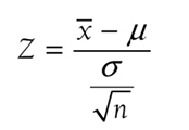
where
x
is the sample mean,
μis the population mean,
σ is the known population standard deviation, and
n is the sample size. So, the test statistics for our example will be
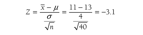
based on data showing that the average number of falls for 40 participants was 11. Given the test statistic of μ3.1, the p-value will be the probability to the left of μ3.1 and is .001 from Figure 6-18.
Step 5: Use the p-Value to Quantify Evidence Against the Null HypothesisNote we had a p-value of .001 associated with the test statistic of μ3.1. Conventionally, we would have compared this p-value against an arbitrarily chosen alpha value such as .05 and concluded that the result was statistically significant. In fact, the p-value is small and would indicate that we would observe the difference as extreme as our statistic in 1 sample out of 1,000, and we will not reject the null hypothesis otherwise. However, whether the result is meaningful is a clinical/practical question, not a statistical one. In other words, it is not the p-value that determines the meaningfulness of the result; rather, it is what is clinically meaningful/effective in terms of what was measured (i.e., the number of falls in this example). So, the result of the average drop of 2 in the average number of falls from 13, with a sample mean of 11, will be meaningful, with p = .001 if it was expected to be clinically meaningful based on researchers’ substantive knowledge.
As discussed earlier, it is important to support the p-value with a measure of effect size, along with a corresponding interval estimate (i.e., confidence interval) as a measure of importance. Let us discuss effect size in general, and then we will come back to how we support the p-value in this example.
Platts-Mills et al. (2012) found that emergency providers reported lower satisfaction with access to resident information in skilled nursing facilities (SNFs) that accept Medicaid (7.13 vs. 8.15, p 0.001) vs. those facilities that did not accept Medicaid. Based on these findings, should SNFs reject Medicaid funding? Can we say with any certainty that Medicaid funding is the cause of lower satisfaction? The answer to both questions is a big “No!” Statistical significance, the p-value, alone does not tell us how much of an effect was present and how important the size of the effect is in practice. Statistical significance has never answered the question of clinical meaningfulness and never will! This is in large part what has driven the aforementioned ASA’s recommendations.
Effect size is the measure of the strength or magnitude of an effect, difference, or relationship between variables. This computation helps us evaluate the clinical importance of study findings. Effect size may be thought of as a doseμresponse curve or rate. We are often exposed to this idea when evaluating how an individual patient responds to medication therapy; that is, different doses of a drug have varying magnitudes of effect. Aspirin prescribed at 80 mg daily has little analgesic effect, but when increased to 650 mg, aspirin has an analgesic effect that is noticeable. We understand that the effect of aspirin differs with the dose. We can measure similar effects of other interventions, including our fall prevention approach. An intervention with a large effect size is more likely to produce the clinical effect that we are looking for. Therefore, effect size allows us to make a more meaningful inference from a sample to a population. Recently, many professional journals have begun to require that investigators report the effect size in their results, and the ASA recommends reporting the effect size along with a corresponding interval estimate—providing us with important information about the clinical significance or importance of the findings.
Types of Effect SizeThere are several ways to compute effect size, including Cohen’s d, Pearson’s r coefficient, ω2, and others. However, we will only discuss Cohen’s d and Pearson’s r, the two most commonly used measures, as an introduction to effect size. We will discuss other types of effect sizes for different types of statistical tests in later chapters.
Cohen’s d is simply the difference of the two population means divided by the standard deviation of the data, and it is shown in the following formula:
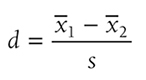
where s is the standard deviation of either group when the variances of the two groups are equal, or
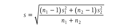
when the variances of the two groups are not equal. Going back to our fall prevention example, we can use Cohen’s d as an effect size for a one-sample z-test, and it will be

Note a value of ±.2 represents a small effect, ±.5 represents a medium effect, and ±.8 represents a large effect for Cohen’s d (Cohen, 1988), so our result shows a medium effect, with a 95% confidence interval [9.76, 12.24], in the average number of falls. Note that the use of Cohen’s definition for small, medium, and large effect sizes can be misleading. For example, Cohen’s d of 0.8 indicates a large effect size, but this effect size may not mean the same in another type of effect size.
Pearson’s r coefficient allows an examination of the relationship between two variables. It is the easiest coefficient to compute and interpret and can be calculated from many statistics. For example, Pearson’s r coefficient as an effect size can be found by the following equation:
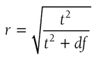
where t is the t-test statistic and df is the degrees of freedom. Details of these two statistics will be discussed in Chapter 11. The value varies between -1 and +1, and the effect size is small if the value varies around 0.1, medium if the value varies around 0.3, and large if the value varies around 0.5.
Meaning and InterpretationEffect sizes are important because they are an objective measure of how large an effect was in a study, and they allow the nurse to consider the practical/clinical importance through the magnitude of the effect that the statistical inference cannot tell us.
As many researchers have noted the issues related to p-values, it is possible that a traditional statistically significant result may not be practically or clinically significant, and a statistically nonsignificant result may be practically or clinically significant (Gelman, 2015; Ioannidis, 2005; Ioannidis, 2019; Nuzzo, 2014). For example, a study may be statistically nonsignificant because of a small sample size, and yet demonstrate a large effect size of a newly developed intervention for preventing central lineμassociated bloodstream infections. Or, a study may have had a statistically significant result because of an excessively large sample size, and yet have such a small effect size that application to individual patients is not possible. The practical/clinical importance of the study should be determined with careful consideration of the sample size and the purpose of the study.
Remember, we are not completely eliminating the use of p-values. Rather, we will use p-values to quantify evidence against the null hypothesis and support it with effect size as a measure of importance.
Statistical power is the probability of rejecting the null hypothesis when it is false, or of correctly saying there is an effect when it exists. Remember that a Type II error (β) is the probability of not rejecting a null hypothesis when it is false, or of reporting no difference in effect when there actually is one. Therefore, statistical power is equal to 1 μβ. From this equation, we can see that statistical power increases as the Type II error decreases, and we would want to obtain higher statistical power for the sake of our confidence in making the right conclusions.
Factors Influencing PowerHigher power is desirable in most situations, and there are several factors that can influence statistical power, including the level of significance, effect size, sample size, and the type of statistical test. The level of significance is the designated probability of making a Type I error, and you will generally obtain the greatest statistical power when you increase the level of significance because Type I error and Type II error are in an inverse relationship and the power is 1 μβ.
Effect size is the magnitude of the relationship or difference found in a hypothesis test. When hypothesis testing produces a small p-value for a relationship or difference, it does not tell us how big the effect, relationship, or difference is—all that a small p-value says is that there is a relationship or difference. For example, the small p-value, such as .001, result we found with our two-tailed fall prevention example only tells us that the average number of falls is likely to be different from 13; it does not calculate the magnitude of the difference between the approaches. However, the effect size tells us the clinical importance of a statistical finding. In general, the statistical power increases as the effect size increases.
Statistical power also increases as the sample size increases. When the sample size is small, our chance of accurately representing the population is low, and the results may not be generalizable. Therefore, the probability of making the correct decision against the null hypothesis is low. The larger the sample, the more likely that the sample will represent the population and the higher the probability of making the correct decision.
The last factor, the type of statistical test, will also influence the probability of rejecting the null hypothesis. In general, more complex statistical tests will require a larger sample size.
Types of Power AnalysisPower analyses are performed to determine the requirements to reject the null hypothesis when it should be rejected. You can conduct power analyses before or after the study is completed. A power analysis conducted before the study is completed is called an a priori power analysis, and it is a guide for estimating the sample size required to detect statistical effect and correctly reject the null hypothesis. A post hoc power analysis is conducted after the study is completed, and it tells you what level of power the study was conducted at with the obtained sample size, along with other factors. Although post hoc analysis is an option, investigators usually conduct an a priori power analysis, as it is problematic to find out that the study has low power after the study is completed. Most investigators take the minimum power of 0.80 as acceptable for their tests (i.e., there should be a less than 20% chance of committing a Type II error).
Meaning and InterpretationsStatistical power is the probability of rejecting a false null hypothesis or correctly saying there is an effect when it exists, and is stated as a probability between 0 and 1. In other words, statistical power tells us how often we can correctly reject a null hypothesis and say there is a true effect, relationship, or difference. In interpreting the results of any study, how much power the study had in detecting an effect if the effect exists should be carefully considered.
Suppose an investigator wanted to determine whether ownership of hospitals (private vs. public) is related to the frequency of surgical mistakes. The investigator recruited a sample size of 104 to obtain 80% power, suggested by an a priori power analysis. If there is an actual difference in the numbers of surgical mistakes between public and private hospitals, it implies that this study will observe meaningful results in 80% of studies and fail to do so in the other 20% of studies.
Results from a study without enough power should be interpreted with caution, and additional studies with larger sample sizes to increase the statistical power will be required before concluding that there was an effect.
Hypothesis testing allows researchers and clinicians to make informed decisions about the nature of research, evidence-based practice, and quality/process improvement study results by incorporating the probability of the decision being true into the decision-making process. Hypothesis testing involves five general steps: (1) stating hypotheses, (2) proposing an appropriate test, (3) checking assumptions of the chosen test, (4) computing the test statistics (finding the p-value), and (5) using the p-value to quantify evidence against the null hypothesis.
Two hypotheses, the null and alternative hypotheses, are formulated, and these are two competing statements. The hypothesis with no effects is the null hypothesis, denoted as H0, and the hypothesis with an effect is the alternative hypothesis, denoted as H1 or Ha.
Hypothesis testing can be either a one- or two-tailed test of inference. Two-tailed tests of inference determine only whether there is an effect, relationship, or difference, but one-tailed tests also determine the direction of the effect relationship, or difference.
Because a sample is used to make inferences about the population, there will always be a chance of making errors. In hypothesis testing, there are Type I and Type II errors. Type I error is the probability of rejecting a true null hypothesis, and Type II error is the probability of not rejecting a false null hypothesis. The investigator can influence error making by selecting an acceptable sample size.
Effect size is the measure of strength or magnitude of an effect, difference, or relationship between variables. Effect size allows us to evaluate objectively the practical or clinical worth of an intervention, relationship between variables, or difference between groups separately from the statistical significance.
Statistical power is the probability of rejecting a null hypothesis when it is false and equal to 1 - β. Factors such as the level of significance, effect size, sample size, and the type of statistical test affect statistical power. An a priori power analysis helps in determining sample size, given a desired power level (e.g., 0.80), and a post hoc power analysis helps in determining the power of specific statistical tests, given a sample size.
Cohen, J. (1988). Statistical power analysis for the behavioral sciences (2nd ed.). Hillsdale, NJ: Erlbaum.
Gelman, A. (2015). Statistics and the crisis of scientific replication. Significance, (3), 23μ25.
Hayat, M. J., Staggs, V. S., Schwartz, T. A., Higgins, M., Azuero, A., Budhathoki, C., Chandrasekhar, R., Cook, P., Cramer, E., Dietrich, M. S., Garnier-Villarreal, M., Hanlon, A., He, J., Hu, J., Kim, M. J., Mueller, M., Nolan, J. R., Perkhounkova, Y., Rothers, J., ... Ye, S. (2019). Moving nursing beyond p .05. International journal of nursing studies, , A1-A2. https://doi.org/10.1016/j.ijnurstu.2019.05.012
Ioannidis, J. P. (2005). Why most published research findings are false. PLoS Medicine, (8), e124.
Ioannidis, J. P. (2019). What have we (not) learned from millions of scientific papers with P values? The American Statistician, (supp1), 20μ25.
Lucas, R., Zhang, Y., Walsh, S. J., Evans, H., Young, E., &Starkweather, A. (2019). Efficacy of a breastfeeding pain self-management intervention: A pilot randomized controlled trial. Nursing Research, (2), E1μE10.
Nuzzo, R. (2014). Statistical errors: P values, the ‘gold standard’ of statistical validity, are not as reliable as many scientists assume. Nature, (7487), 150μ153.
Platts-Mills, T. F., Biese, K., LaMantia, M., Zamora, Z., Patel, L. N., McCall, B., Egbulefu, F., Busby-Whitehead, J., Cairns, C. B., &Kizer, J. S. (2012). Nursing home revenue source and information availability during the emergency department evaluation of nursing home residents. Journal of the American Medical Directors Association, (4), 332μ336.
Wasserstein, R. L., Schirm, A. L., &Lazar, N. A. (2019). Moving to a world beyond “p 0.05.” The American Statistician, (1), 1μ19.