In a previous chapter, we saw how one-way ANOVA allowed us to examine group differences on a continuous dependent variable. However, in many studies, there may be another continuous variable that may affect the dependent variable, but is not a variable of interest. These variables are known as covariates and can be included in ANOVA to control for their effect in order to examine the true influence of an independent variable on the dependent variable. For example, we may still be interested in examining the effect of the amount of exercise on a health problem index, but we know that body weight will also affect the health problem index score. We can get a better understanding of the influence of weight if we measure the weight and enter it as a covariate in an ANCOVA design. Such a procedure will allow us to control for the effect of weight and discern the true effect of the amount of exercise on the health problem index.
When we identify covariates that influence the dependent variable and carefully control for them in an ANCOVA, we achieve an important goal: we can explain the variability that we could not explain without the covariates. The unexplained variability is reduced, and the design allows us to examine more accurately the true effect of an independent variable. Similar to a regression analysis, ANCOVA allows us to compute the percentage of variance attributed to the independent variable and the covariates—this process is called “partitioning.” The partitioning of the variability is shown in Figure 12-1.
Partitioning of variability in analysis of covariance (ANCOVA).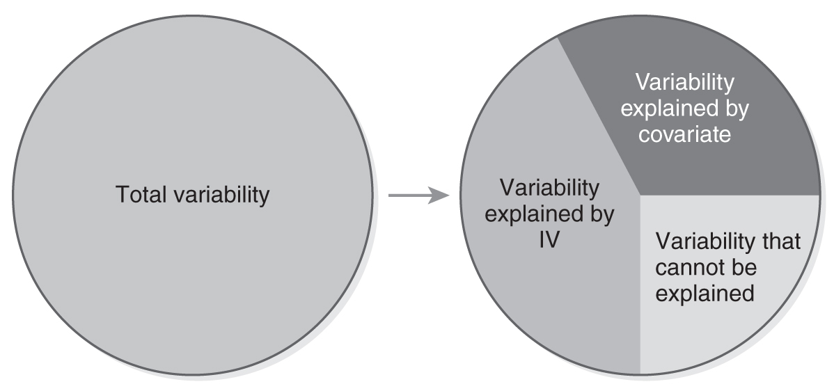
A diagram shows the total variability in ANCOVA, analysis of covariance, partitioned into Variability explained by I V, Variability explained by covariate, and Variability that cannot be explained.
ANCOVA has all of the assumptions of ANOVA, plus an additional two assumptions. These are (1) independence between the covariate and independent variable and (2) homogeneity of regression slope.
Independence between the covariate and independent variable makes sense as we try to reduce the variability that is not explained by the independent variable by explaining it with the covariates. If the covariate and the independent variable are dependent (overlapping), the variability that is computed will be difficult to interpret and it will be unclear whether it was explained by the independent variable.
Homogeneity of regression slope means that the relationship between the covariate and the dependent variable stays the same. For example, the health problem index should increase as the weight increases across all the workout groups.
First, we need to set up hypotheses. These look similar to those of ANOVA design, except the means are adjusted for the covariate:
H0: There is no difference among group means after adjusting for the covariate.
Ha: At least two group means differ after adjusting for the covariate.
or
H0: μ1 = μ2 = μ3 after adjusting for the covariate.
Ha: μj≠μk for some j and k after adjusting for the covariate.
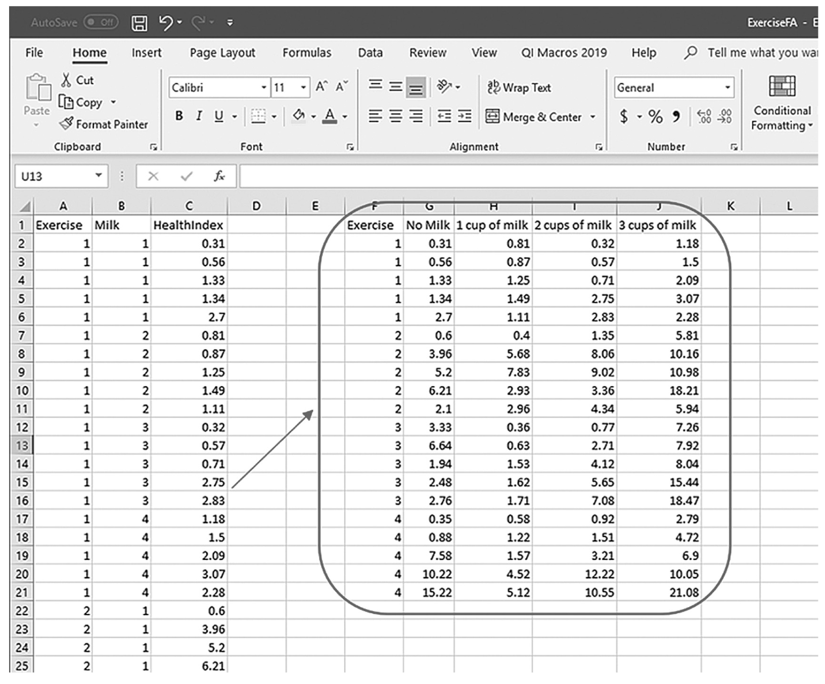
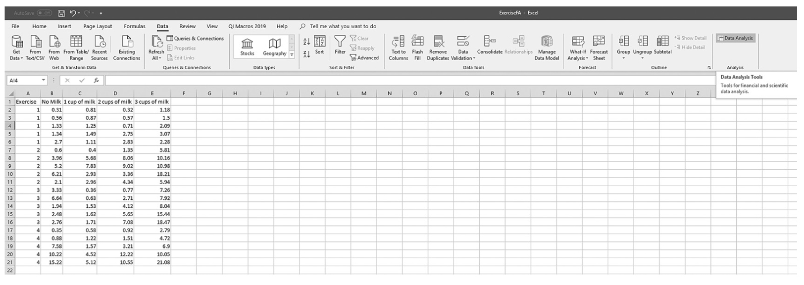
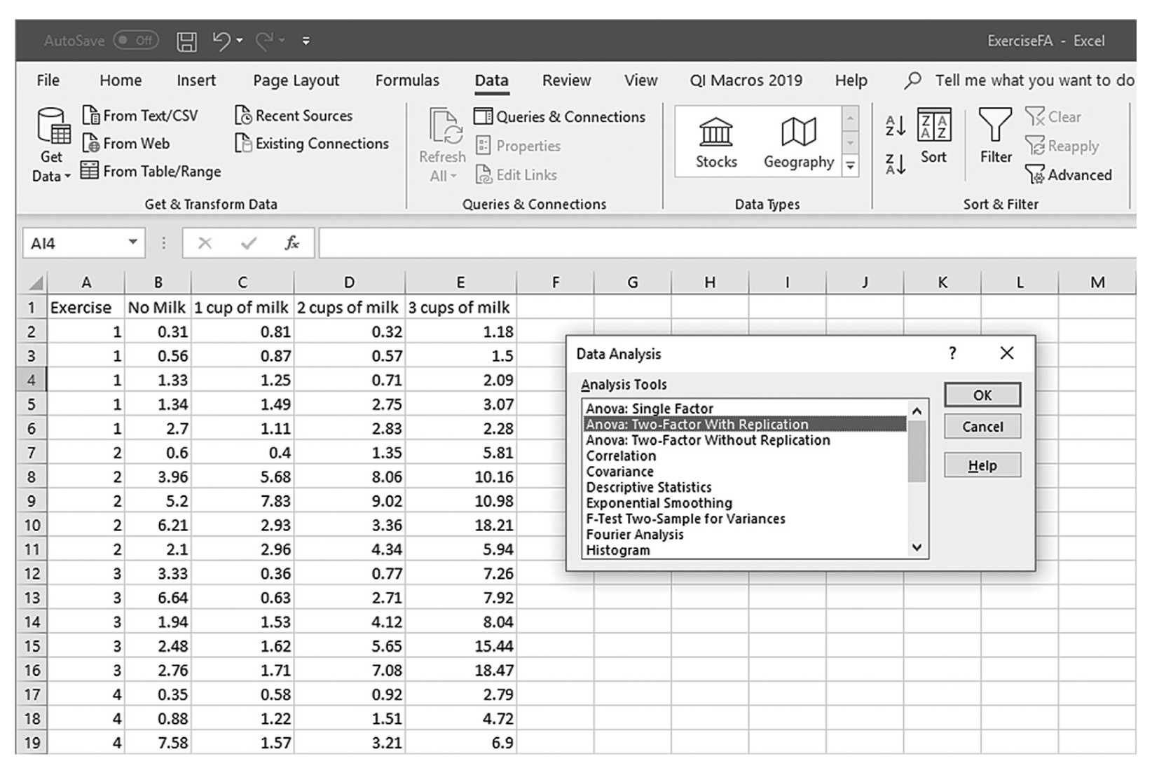
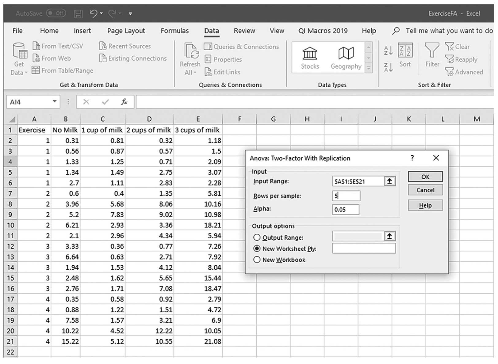
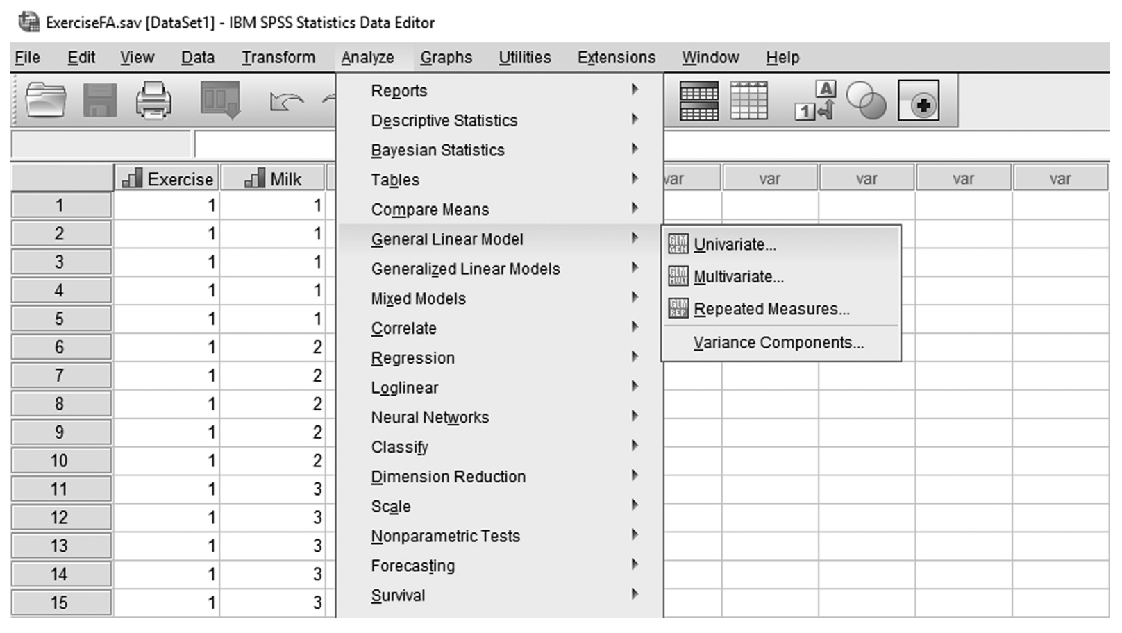
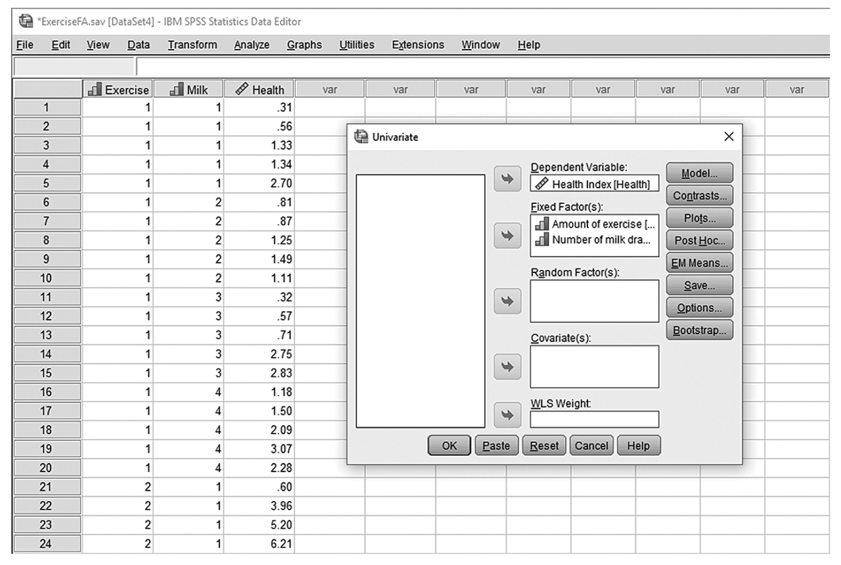
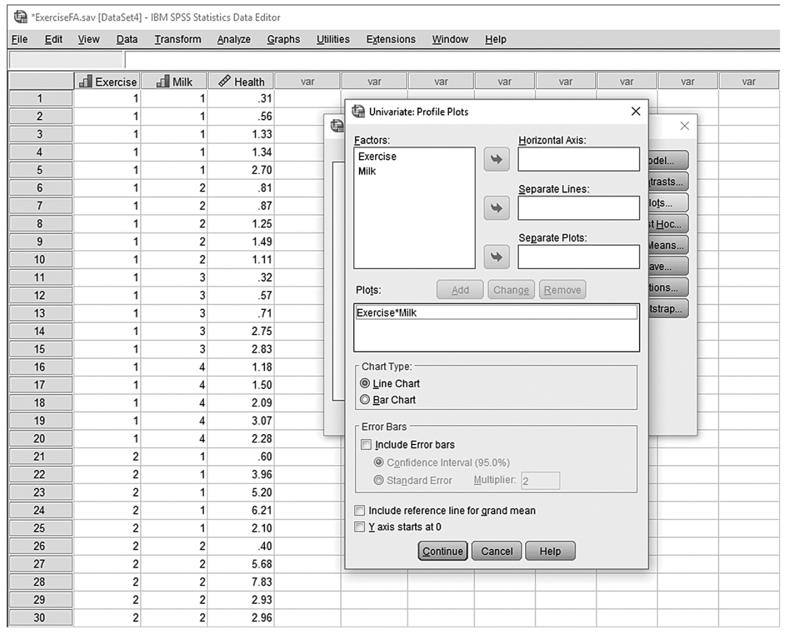
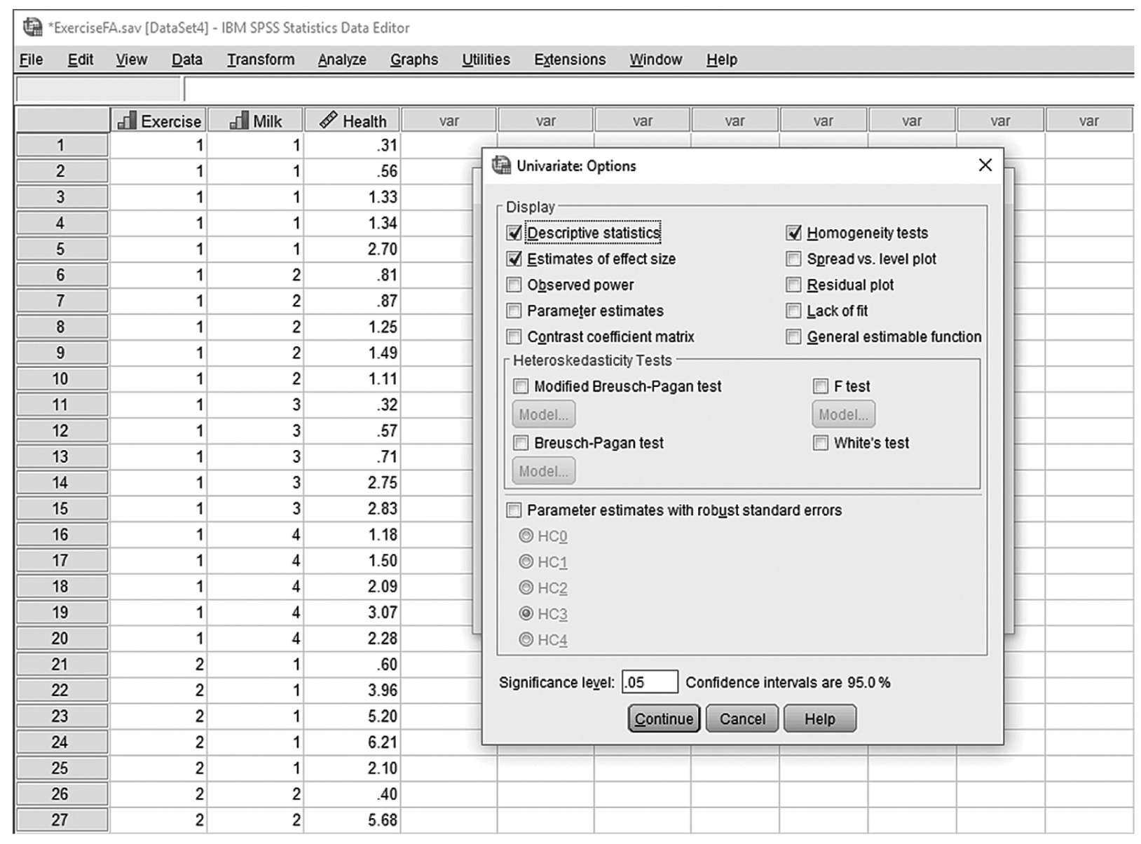
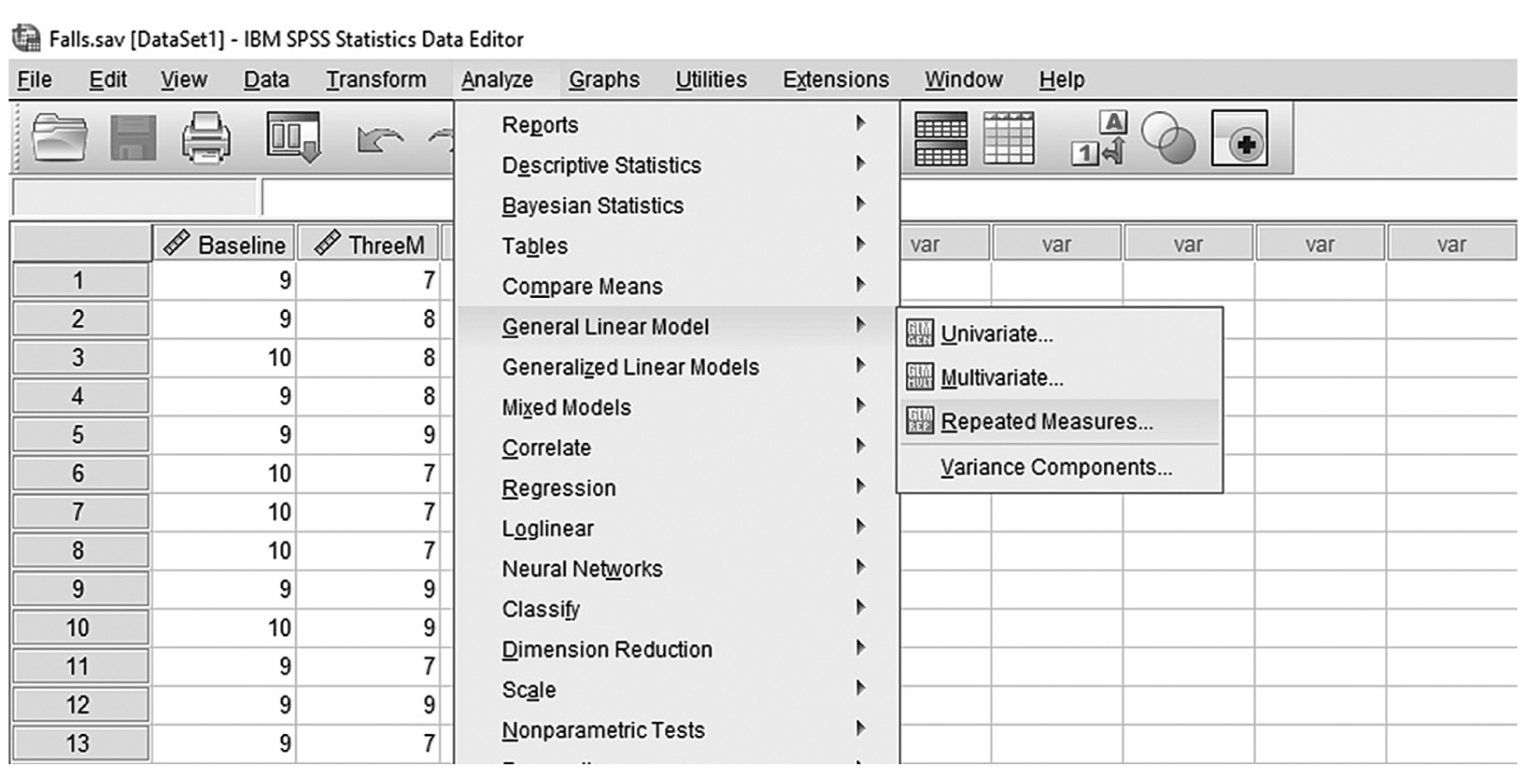
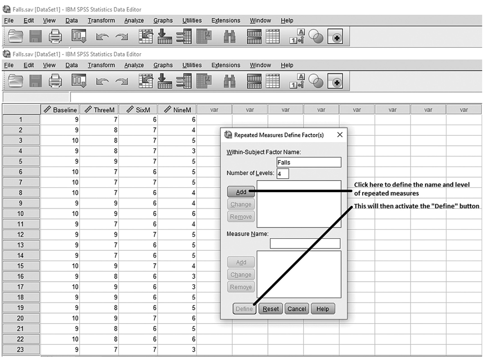
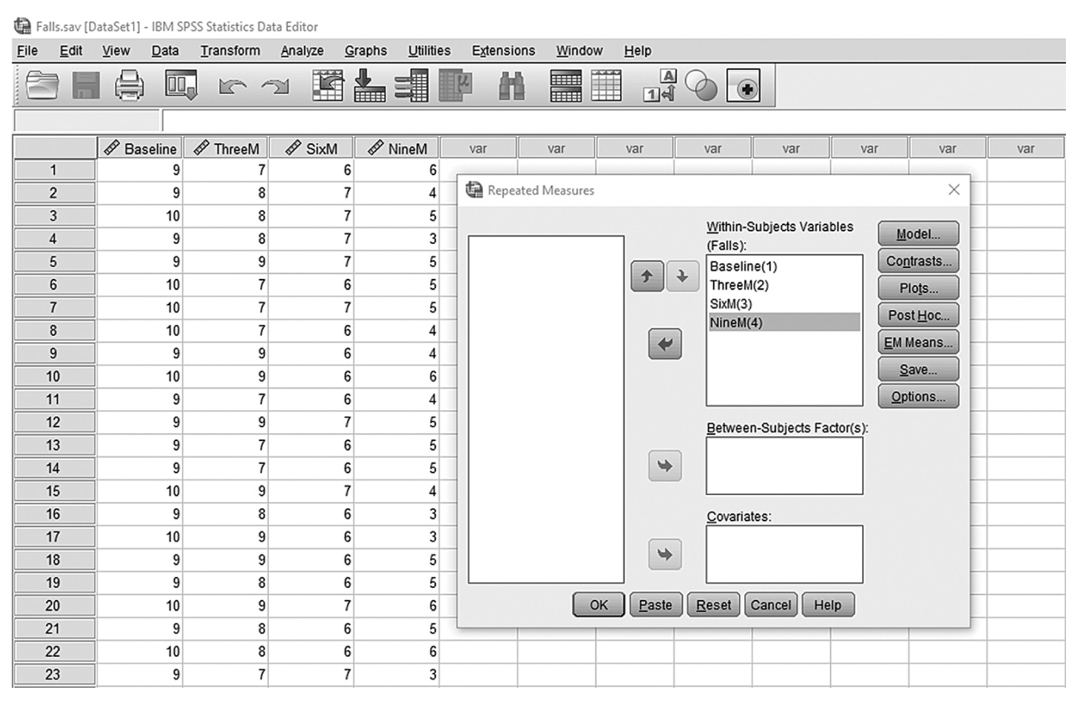
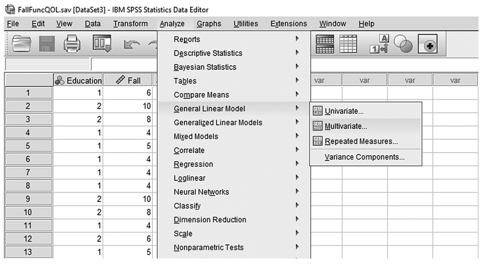
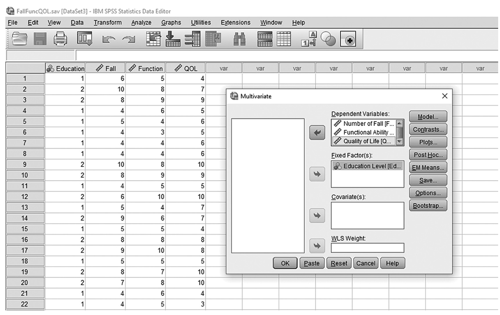
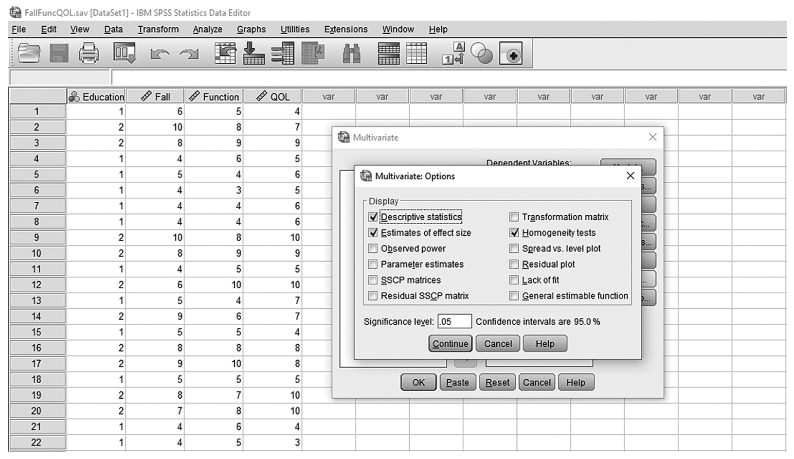
To conduct ANCOVA in IBM SPSS Statistics software (SPSS), you will open ExerciseCov.sav and go to Analyze > Generalized linear models > Univariate, as shown in Figure 12-2. The data here are those we used in the multiple comparison example where the amount of exercise affected the health problem index. In the Univariate dialogue box, you will move the independent variable, Exercise, into “Fixed Factor(s)”; the dependent variable, Health, into “Dependent Variable”; and the covariate, Weight, into “Covariate(s)” by clicking the corresponding “arrow” buttons in the middle, as shown in Figure 12-3. There are six buttons in the box, but only the commonly used buttons are discussed here. The “Contrasts” and “Post Hoc” buttons are used when further investigations are needed among more than two groups in the factor with ANOVA results indicating substantial differences in group means, as discussed in the earlier section on planned contrasts and post hoc tests. The “Options” button gives us several choices that may help us interpret the results of the ANCOVA, and these are shown in Figure 12-4. Please review the example output shown in Table 12-1.
Selecting ANCOVA under “General Linear Models” in SPSS.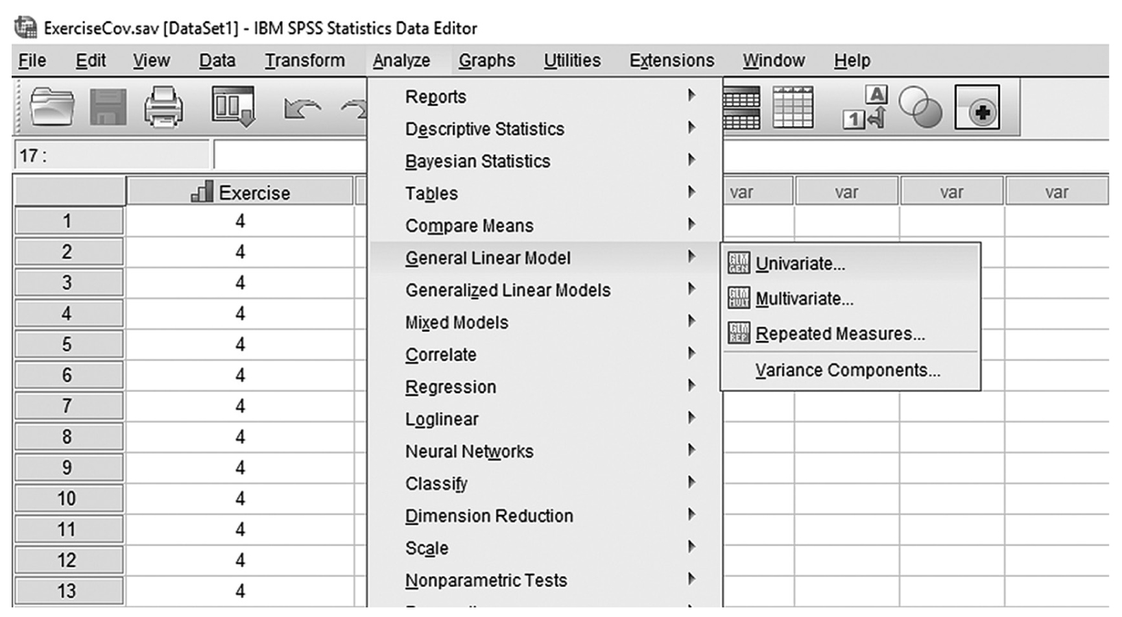
A screenshot in S P S S shows the selection of the Analyze menu, with General linear model command chosen, from which the Univariate option is selected. The data in the worksheet shows columns of numerical data.
Reprint Courtesy of International Business Machines Corporation, © International Business Machines Corporation. “IBM SPSS Statistics software (“SPSS”)”. IBM®, the IBM logo, ibm.com, and SPSS are trademarks or registered trademarks of International Business Machines Corporation.
Defining variables in ANCOVA in SPSS.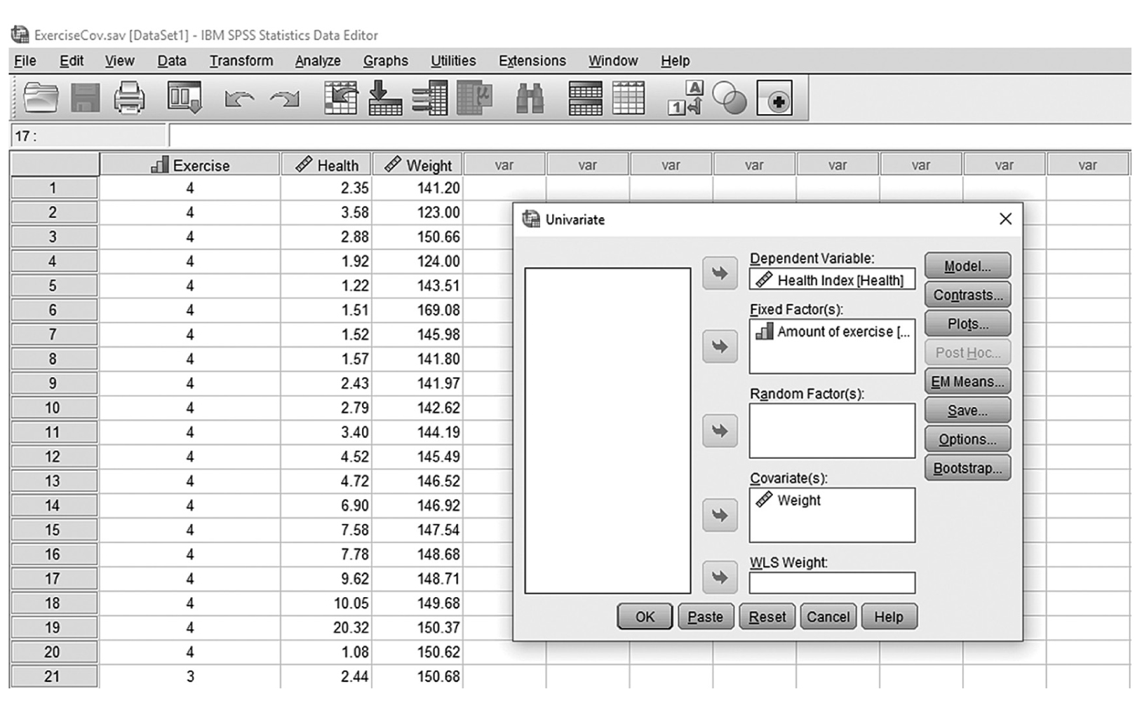
A screenshot in S P S S Editor defines variables in ANCOVA. The numerical data in the worksheet lists Exercise, Health, and Weight values.
Reprint Courtesy of International Business Machines Corporation, © International Business Machines Corporation. “IBM SPSS Statistics software (“SPSS”)”. IBM®, the IBM logo, ibm.com, and SPSS are trademarks or registered trademarks of International Business Machines Corporation.
Useful options for ANCOVA in SPSS.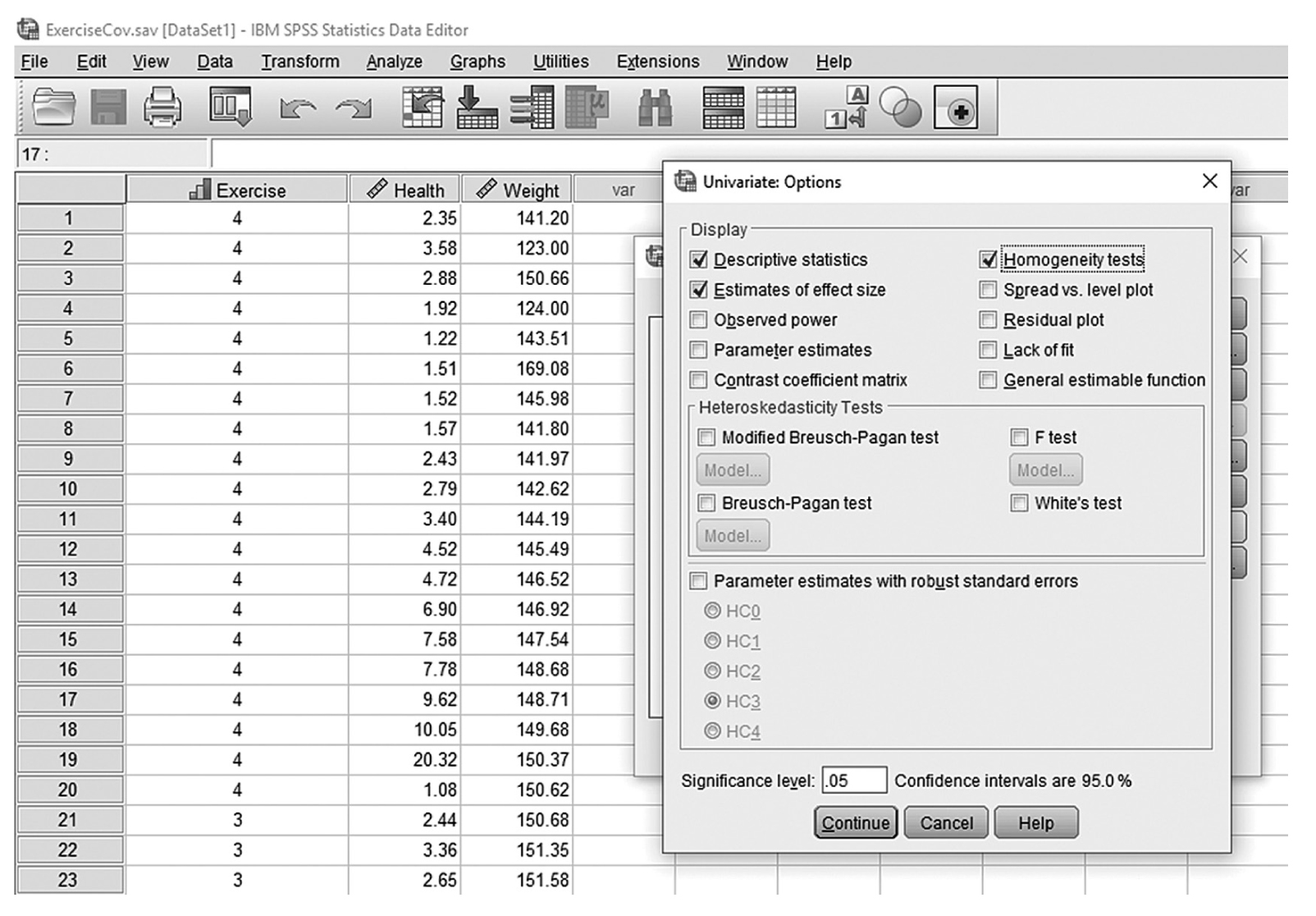
A screenshot in S P S S Editor shows the Univariate Options dialog box. The numerical data in the worksheet lists Exercise, Health, and Weight values.
Reprint Courtesy of International Business Machines Corporation, © International Business Machines Corporation. “IBM SPSS Statistics software (“SPSS”)”. IBM®, the IBM logo, ibm.com, and SPSS are trademarks or registered trademarks of International Business Machines Corporation. Courtesy of IBM SPSS Statistics.
Between-Subjects Factors | |||
|---|---|---|---|
Value Label | N | ||
Amount of exercise | 1 | None | 20 |
2 | 1 day per week | 20 | |
3 | 3 days per week | 20 | |
4 | 5 days per week | 20 | |
Tests of Between-Subjects Effects Dependent Variable: Health Index | |||||
|---|---|---|---|---|---|
Source | Type III Sum of Squares | df | Mean Square | F | Sig. |
Corrected model | 169.937a | 4 | 42.484 | 1.645 | .172 |
Intercept | 112.647 | 1 | 112.647 | 4.363 | .040 |
Weight | 143.437 | 1 | 143.437 | 5.555 | .021 |
Exercise | 163.406 | 3 | 54.469 | 2.110 | .106 |
Error | 1,936.446 | 75 | 25.819 | ||
Total | 3,740.195 | 80 | |||
Corrected total | 2,106.382 | 79 | |||
aR-square (R2) = .081 (adjusted R2 = .032)
You will see that the ANCOVA results table is very similar to that of a one-way ANOVA, but there is an additional line representing the covariate—weight. The result indicates that weight substantially influences the health problem index with a small p-value of .007. However, you will find it interesting that the amount of exercise does not have a substantial effect on the health problem index with the covariate in the design. Do you remember that the amount of exercise made a substantial difference on average health problem index value in one-way ANOVA? When we add the covariate, weight, to our analysis, we find that weight is substantially influencing the health problem index and cancelling out the effect of exercise. If we had neglected to include the covariate of weight, we would have misinterpreted the influence of exercise on the health problem index.
When reporting ANCOVA results, you should report the size of the F-statistics, along with associated degrees of freedom and associated p-value. For an effect size for ANCOVA, omega squared (ω2) can be calculated as it is with one-way ANOVA. Here, ω2 is only useful when the sample sizes for all groups are the same. Another type of effect size, partial eta squared (η2), is useful when sample sizes are not equal, and we can compute this in SPSS.
The following is a sample report from our example:
The covariate, weight, was substantially influencing this sample’s health problem index, F (1, 75) = 5.55, p = .021. However, the amount of exercise per week did not influence the health problem index after controlling for the effect of weight, F (3, 75) = 2.11, p = .106, ω2 = .04.
Further group comparisons of the amount of exercise per week are not considered, as the overall test did not find substantial differences on the average health problem index.