The t-test is the simplest statistic when we are comparing two means, and a one-sample t-test is the simplest t-test. A one-sample t-test compares the mean score of a sample on a continuous dependent variable to a known value, which is usually the population mean. For example, say that we take a sample of students from the university and compare their average IQ to a known average IQ for the university. If we want to find out whether the sample mean IQ differs from the average university IQ, a one-sample t-test will give us the answer.
There are three assumptions for a one-sample t-test:
- We must know the population mean.
- The sample should be randomly selected from the population and the subjects within the sample should be independent of each other (no participant will be sampled/measured more than once).
- The dependent variable should be continuous and normally distributed.
Always remember to check these assumptions before you conduct the test as violations can limit scientific conclusions.
As with all hypotheses testing, we need to first set up the hypotheses:
H0: There is no difference between the sample mean and a known population mean.
Ha: There is a difference between the sample mean and a known population mean.
or
H0: μ= 120
Ha: μ≠120.
The test statistic for a one-sample t-test can be computed by using the following formula:

where
x
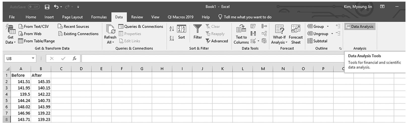
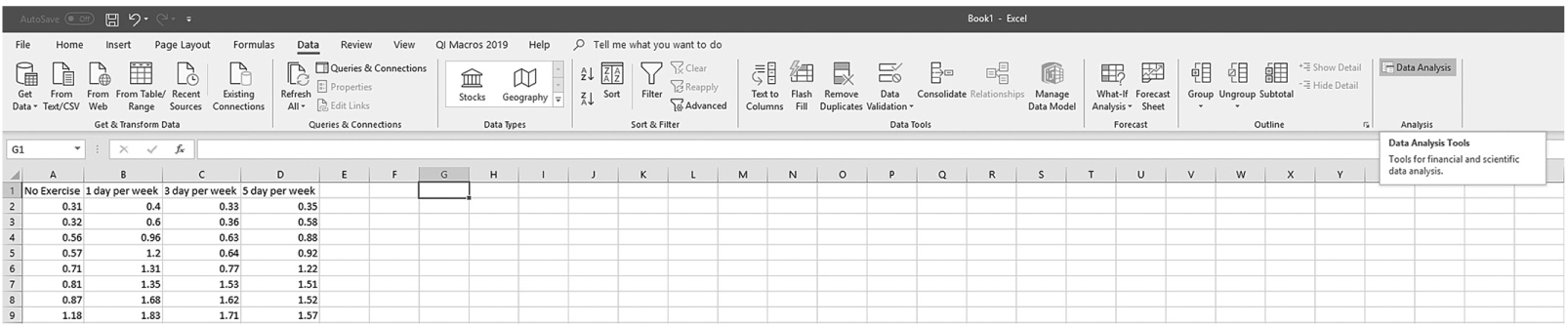
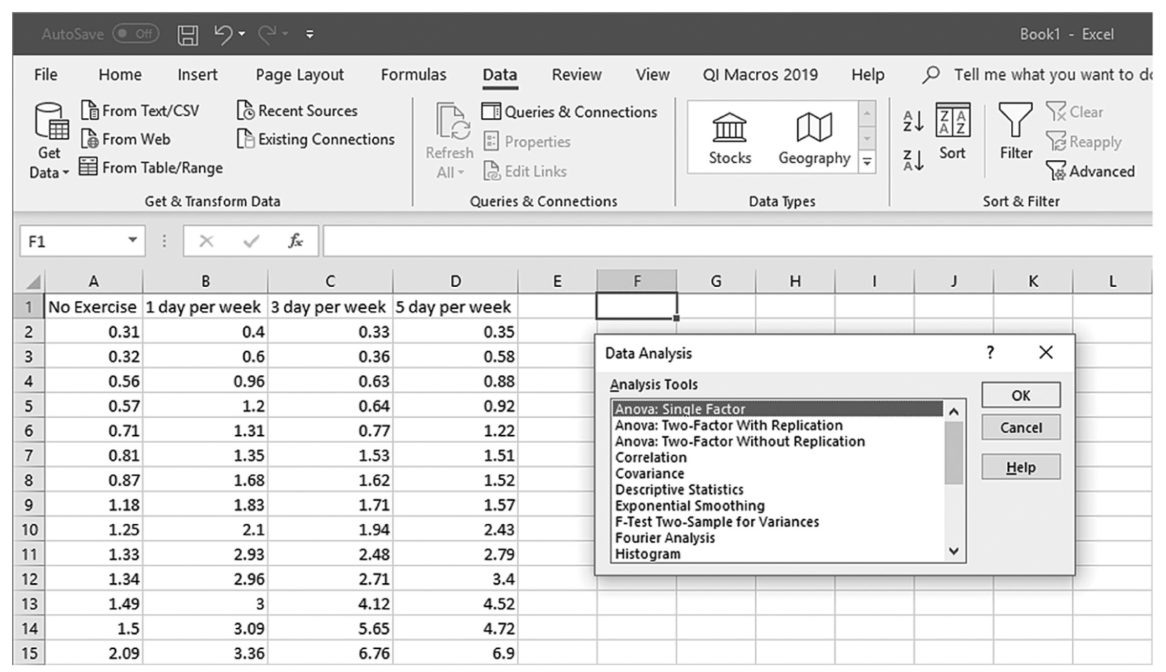
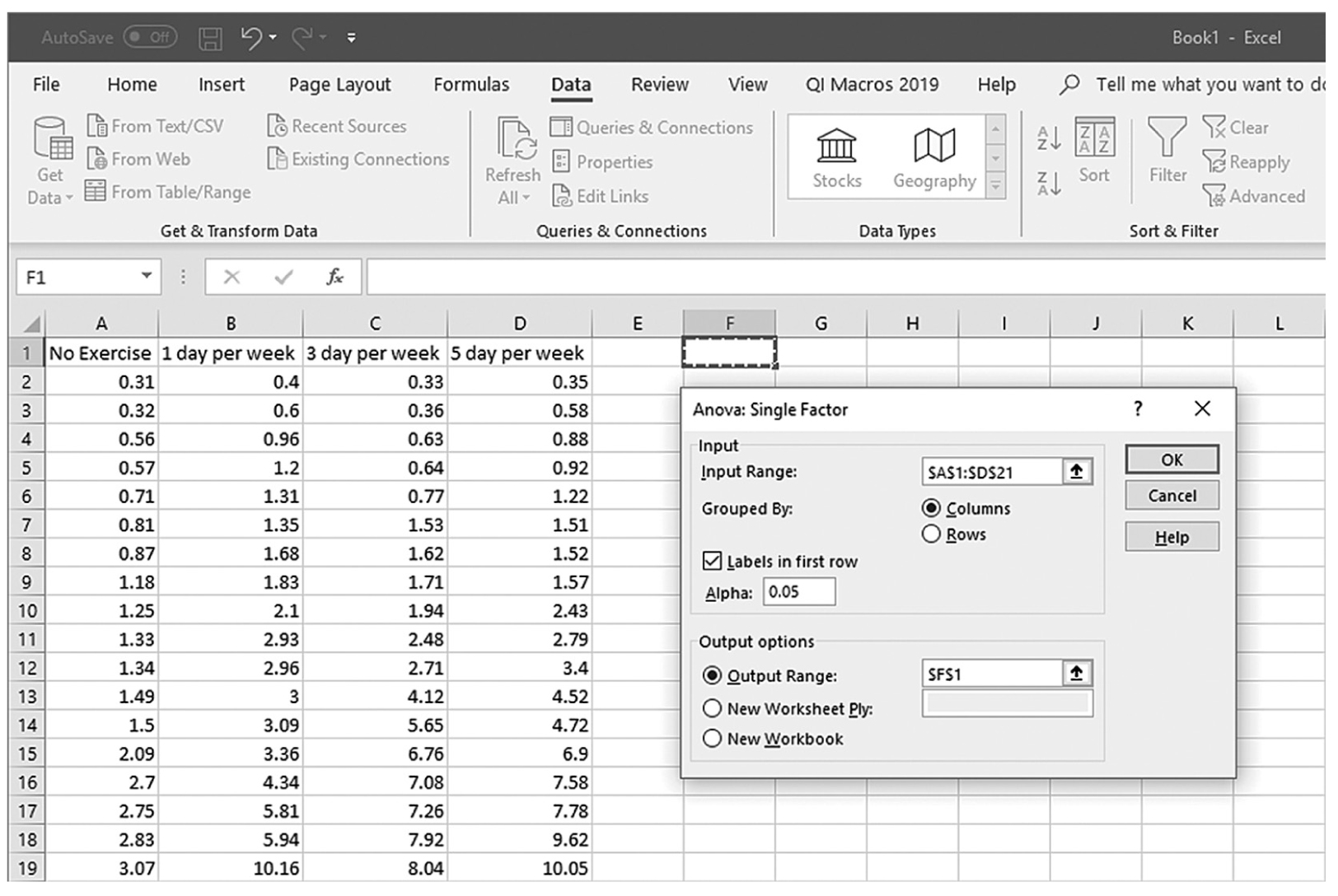
is the sample mean, μis the population mean, s is the sample standard deviation, and n is the sample size. Then we report the associated p-value with the computed statistic and support the p-value with a measure of effect size along with a corresponding interval estimate (i.e., confidence interval) as a measure of importance.To conduct a one-sample t-test in Excel, you will open IQ.xlsx and go to Data > Data Analysis, as shown in Figure 11-1. Note that the list does not include one-sample t-test, but you can trick Excel and perform a one-sample t-test. First, you will type the word Average in cell B1, which is our label for a known population mean, and a known population mean, 120, in cells B2 and B3 (Figure 11-2). In the Data Analysis window, choose “t-Test: Two-Sample Assuming Unequal Variances” and then click “OK” (Figure 11-3). In the “t-Test: Two-Sample Assuming Unequal Variances” box, you will provide A1:A101 as Variable 1 Range and B1:B3 as Variable 2 Range with Labels selected (Figure 11-4). Clicking “OK” will then produce the output of the requested one-sample t-test; the example output is shown in Figure 11-5.
Finding Data Analysis ToolPak in Excel.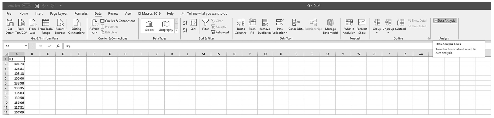
An Excel screenshot shows the Data Analysis ToolPak add-in, in the Analysis group under Data menu.
Courtesy of Microsoft Excel © Microsoft 2020.
Preparing the data for Excel to compute a one-sample t-test.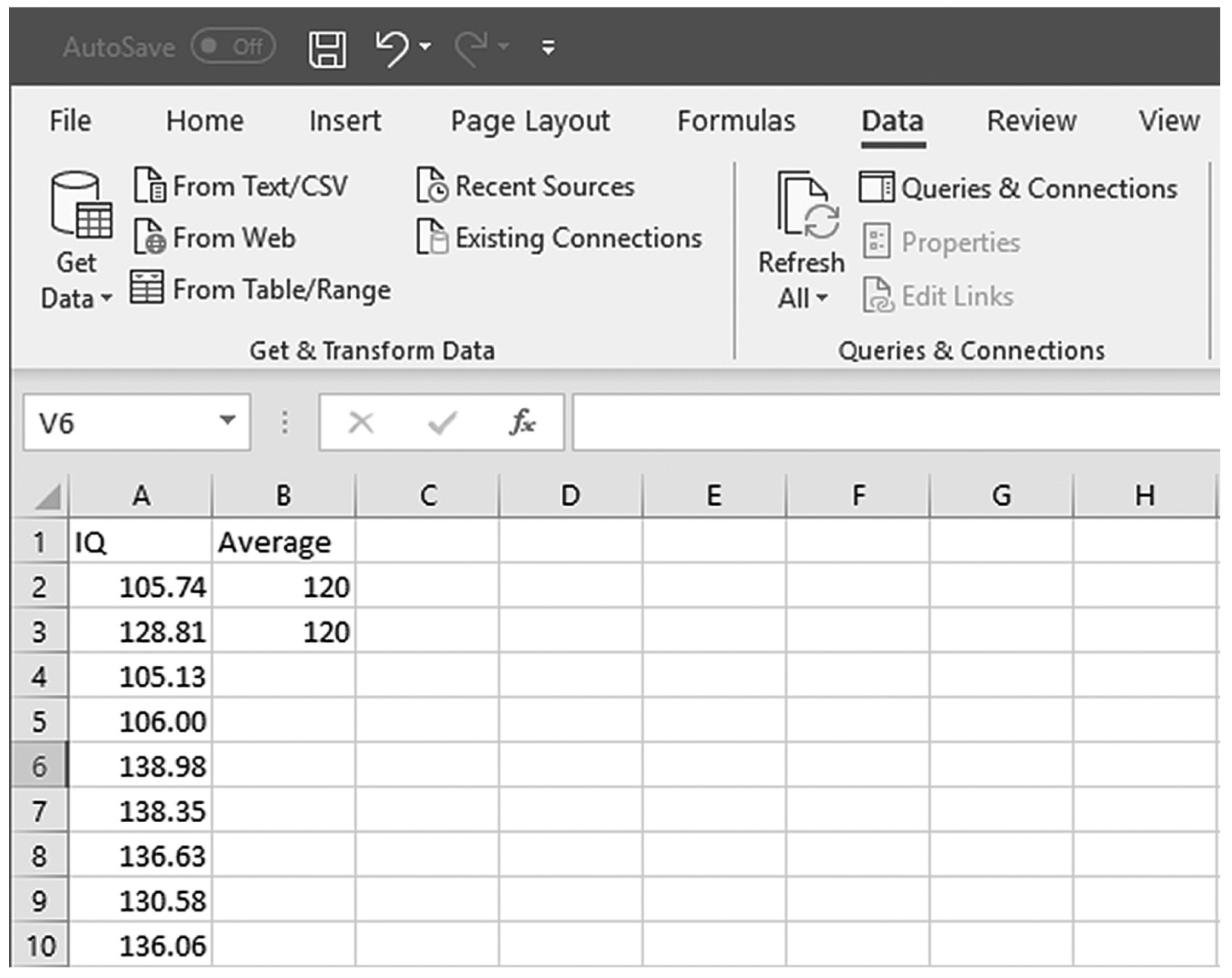
An Excel screenshot shows the column heading, I Q, in cell A 1, and numerical data entered in cells A 2 through A 10. The column heading, Average, is entered in cell B 1, and the value 120, entered in cells B 2 and B 3.
Courtesy of Microsoft Excel © Microsoft 2020.
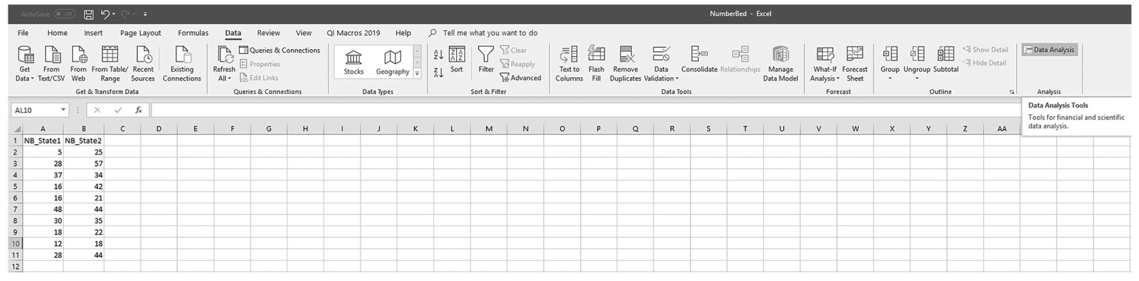
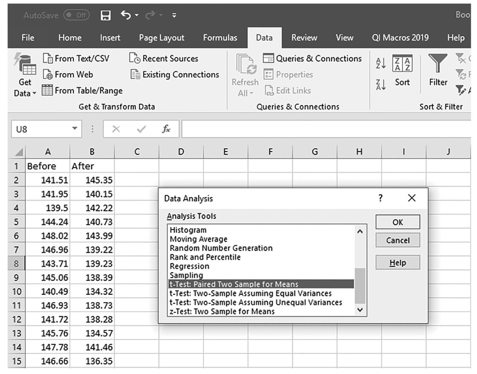
Selecting a one-sample t-test within the Data Analysis ToolPak list in Excel.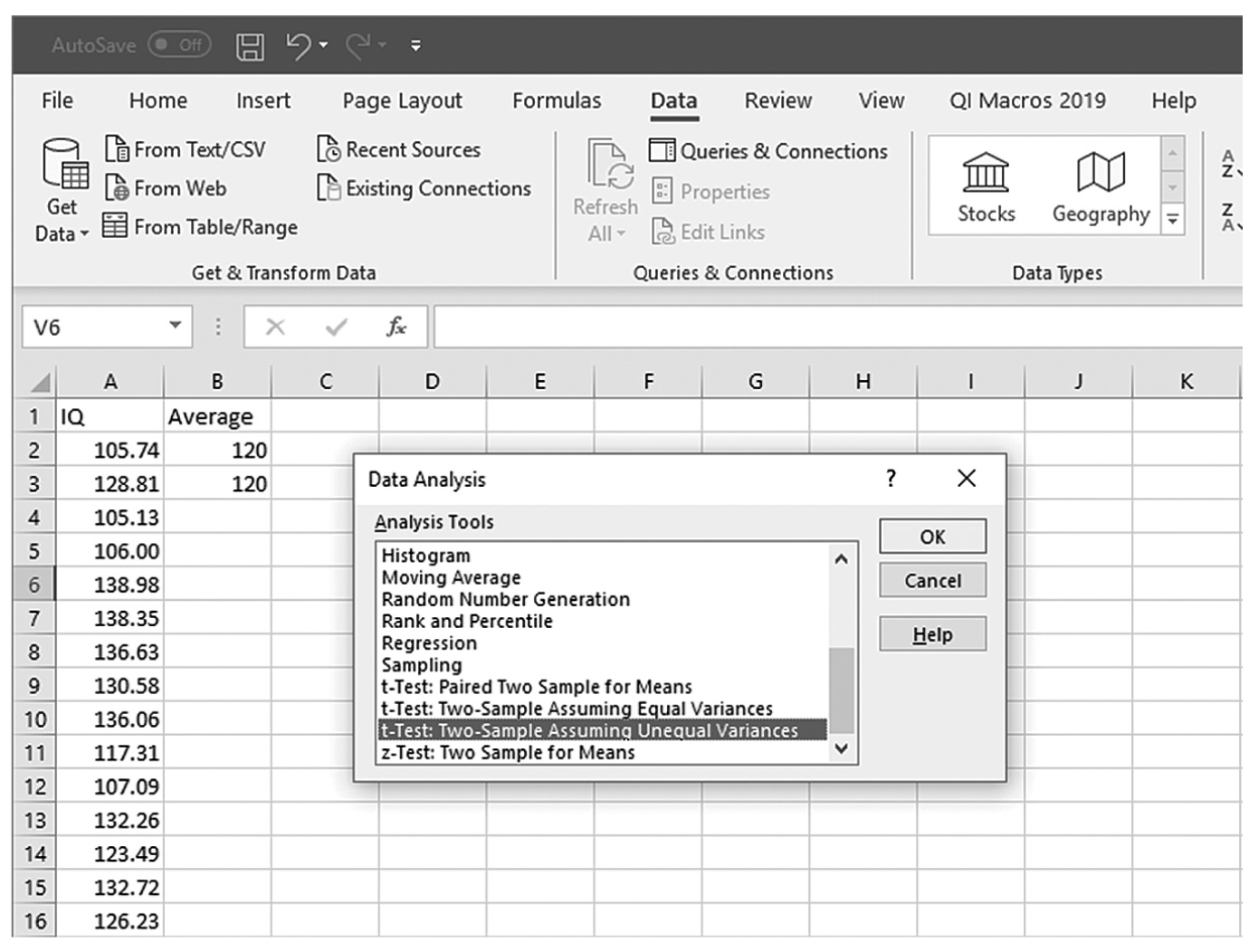
An Excel screenshot shows selection of the option, t-Test: Two-Sample Assuming Unequal Variances, within the Data Analysis ToolPak. The worksheet lists I Q with numerical data, and Average with the value 120 entered below it.
Courtesy of Microsoft Excel © Microsoft 2020.
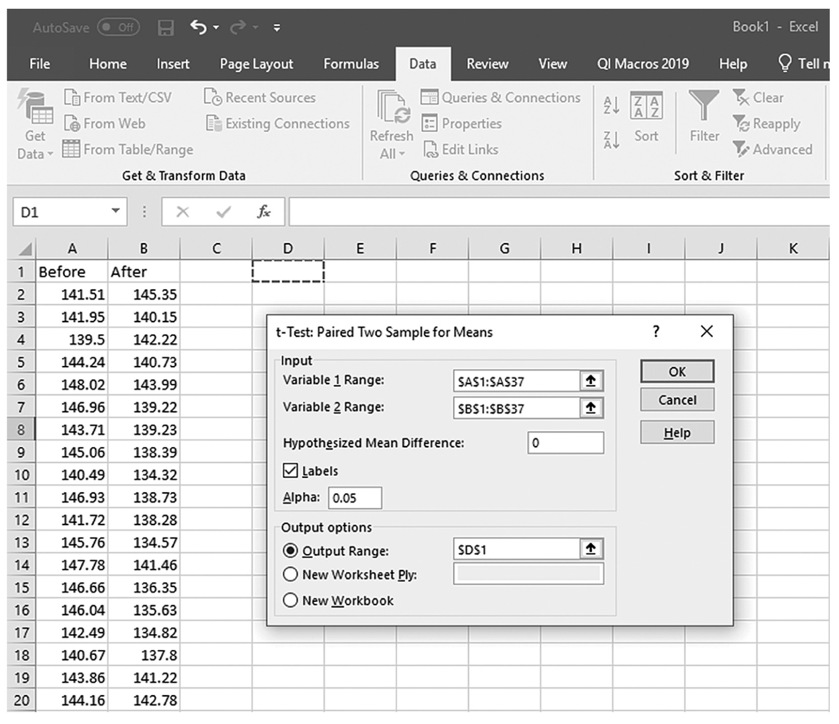
Defining data ranges and selecting options for a one-sample t-test in Excel.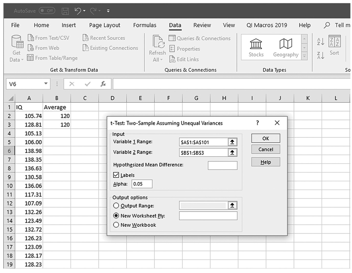
An Excel screenshot shows a dialog box with the inputting of data ranges and selecting output options for a one-sample t-test. The worksheet lists I Q with numerical data, and Average with the value 120 entered below it.
Courtesy of Microsoft Excel © Microsoft 2020.
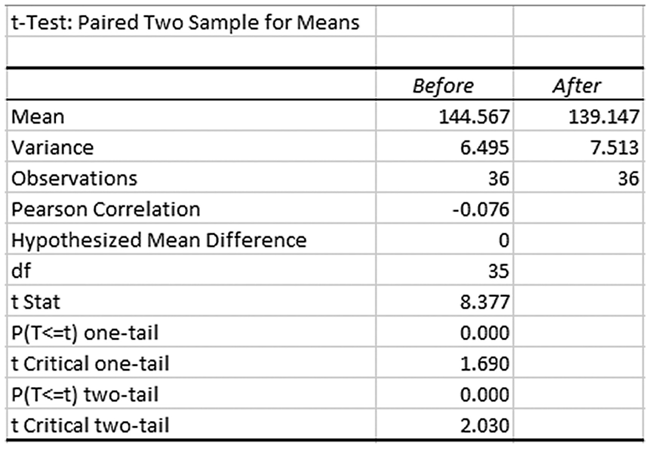
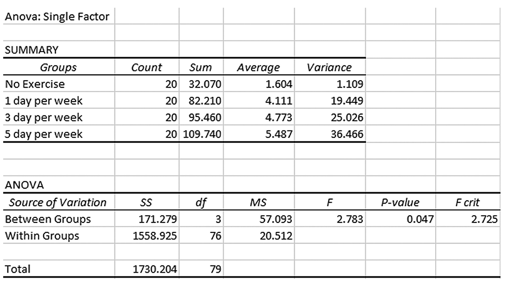
Example output for a one-sample t-test in Excel.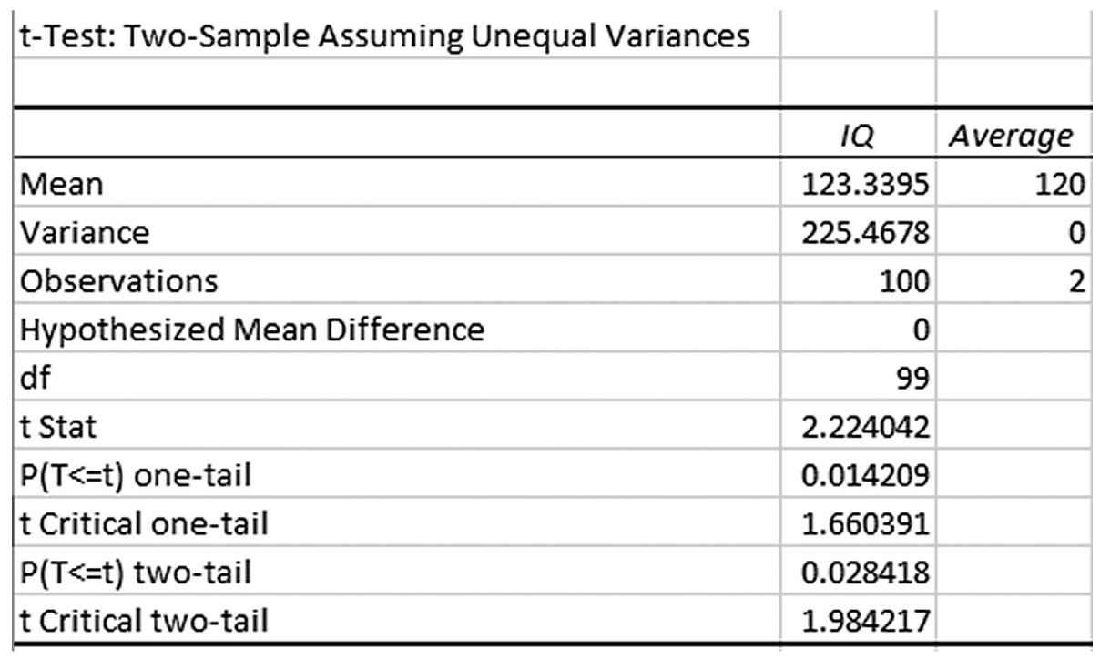
An Excel screenshot displays the output for a one-sample t-test.
Courtesy of Microsoft Excel © Microsoft 2020.
You see that the average IQ of our sample was 123.34 and the t-statistic and corresponding p-value are 2.224 and .028, respectively. A small p-value of .028 indicates that the observed difference between the sample mean and a known population mean of 3.34 units was large enough to rule out chance.
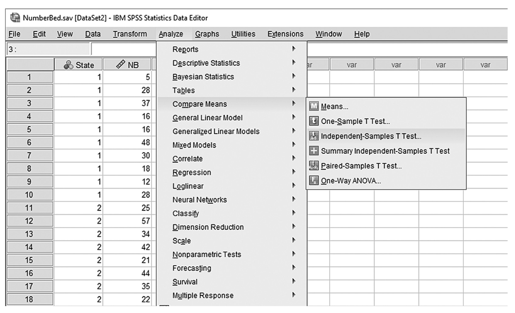
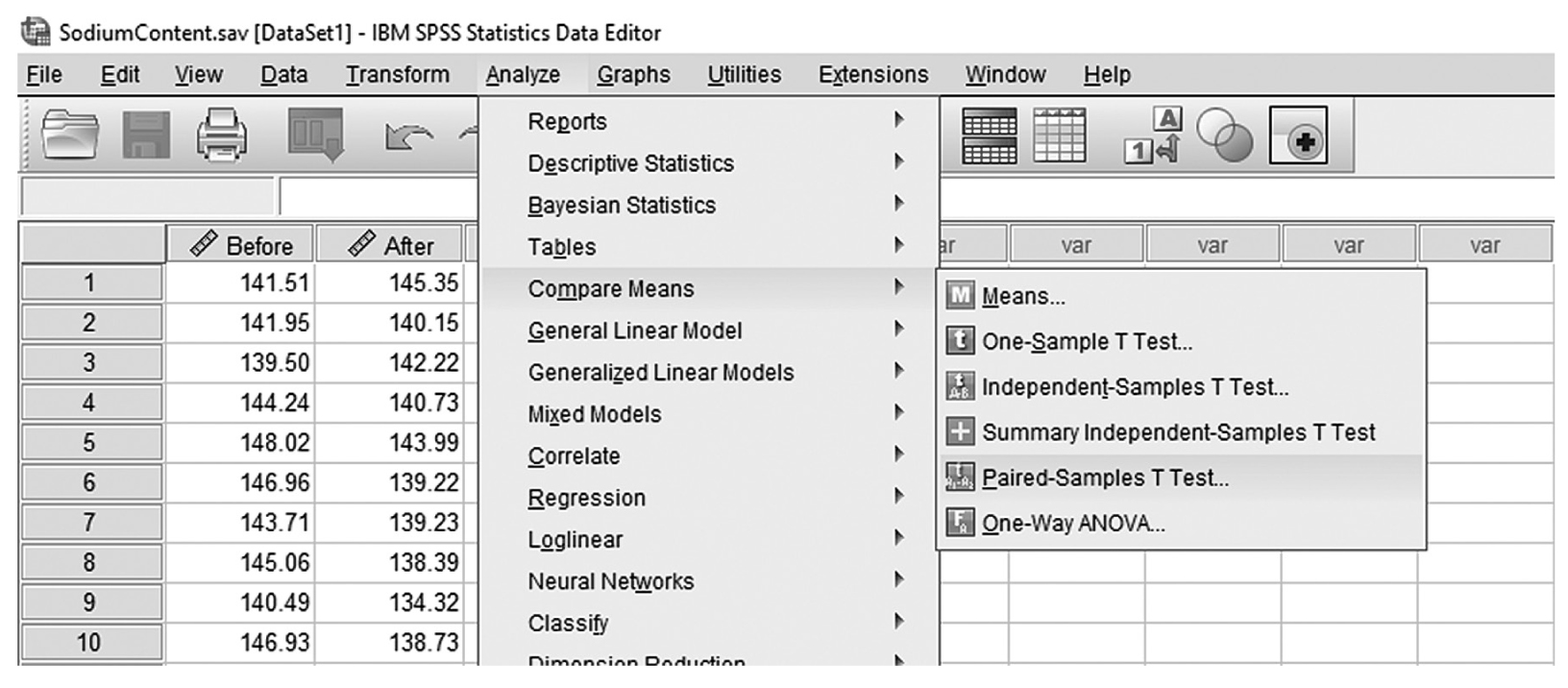
To conduct a one-sample t-test in IBM SPSS Statistics software (SPSS), you will open IQ.sav and go to Analyze > Compare means > One-sample t-test, as shown in Figure 11-6, in this case using IQ measurements from a sample of nursing students. In the One-Sample t-Test dialogue box, you will move IQ into “Test Variable(s)” by clicking on the arrow buttons in the middle and typing in a known population mean (in this case, 120), into “Test Value” (Figure 11-7).
Selecting a one-sample t-test in SPSS.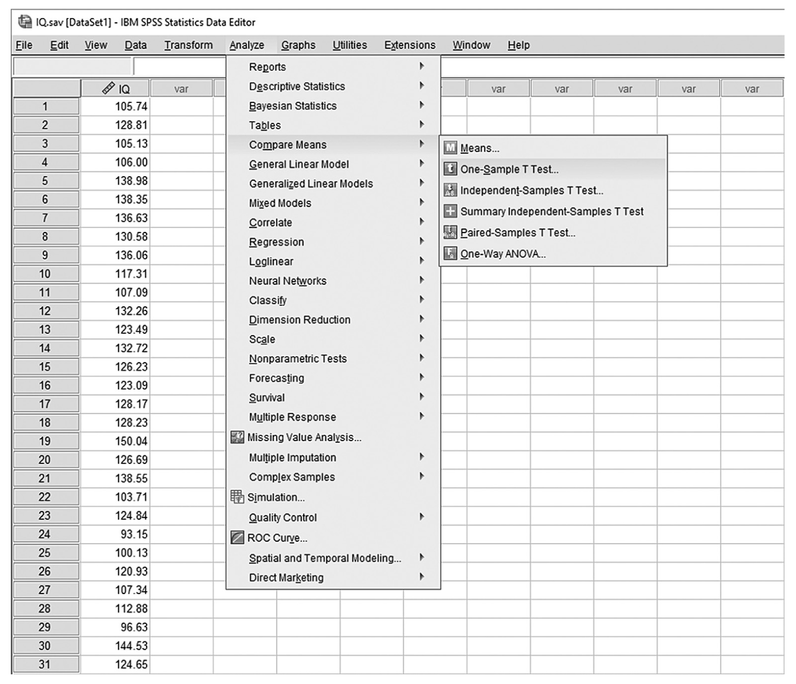
A screenshot in S P S S shows the selection of the Analyze menu, with Compare means command chosen, from which the One-sample t-test option is selected. The data in the worksheet shows a column of numerical data.
Reprint Courtesy of International Business Machines Corporation, © International Business Machines Corporation. "IBM SPSS Statistics software ("SPSS")". IBM®, the IBM logo, ibm.com, and SPSS are trademarks or registered trademarks of International Business Machines Corporation Courtesy of IBM SPSS Statistics.
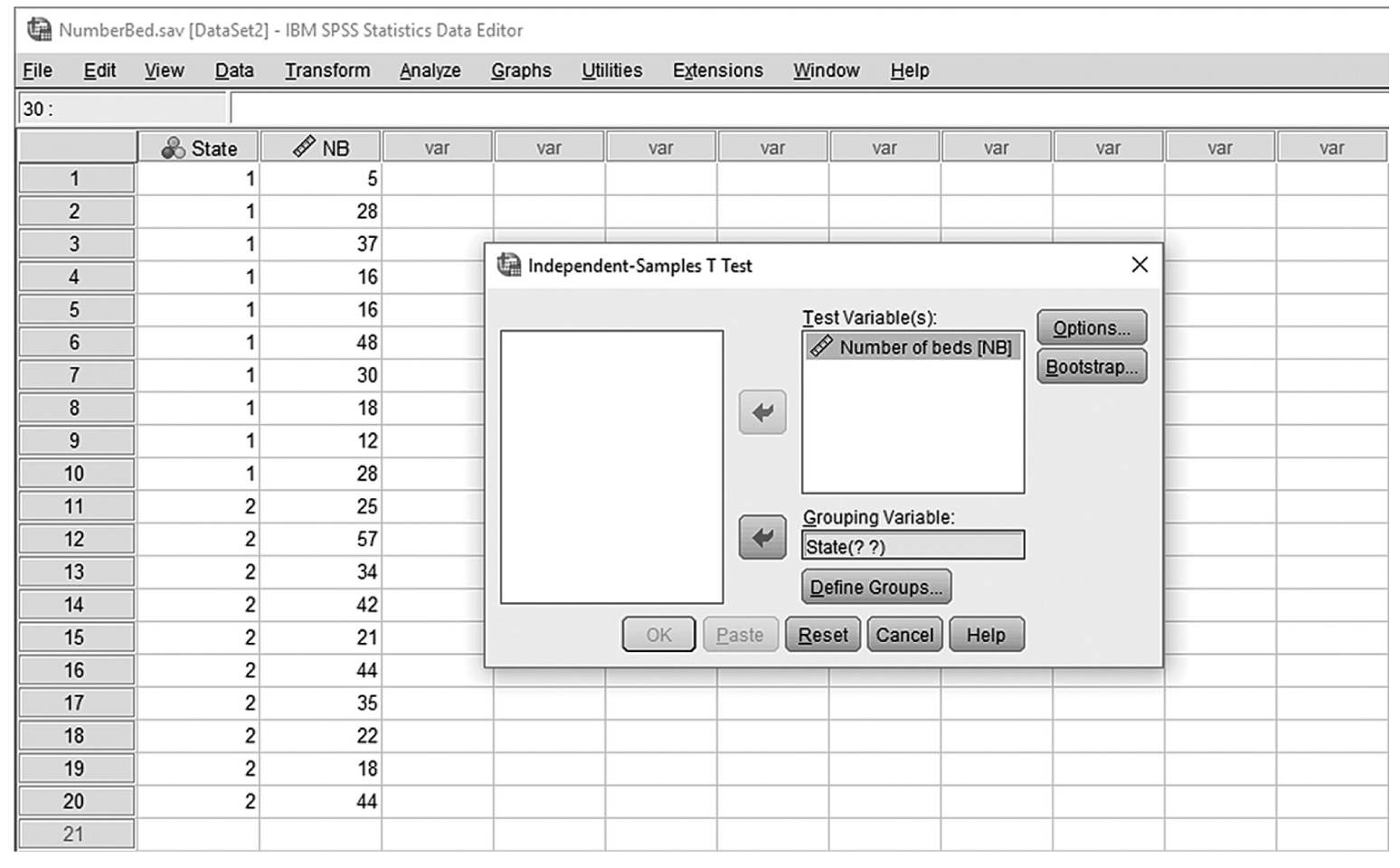
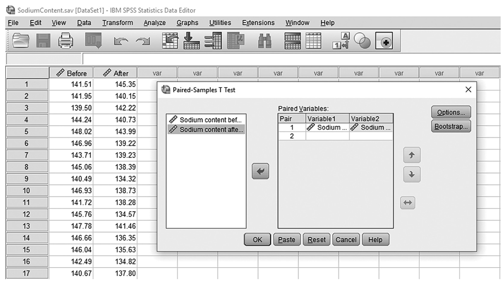
Defining variables in a one-sample t-test in SPSS.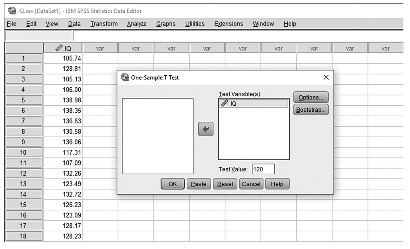
A screenshot in S P S S shows a dialog box with heading, One-sample t-test. Variable I Q is defined in Test variable box. Test value field shows 120. Buttons, Options and Bootstrap, are on right side; Ok, Paste, Reset, Cancel, and Help at the bottom.
Reprint Courtesy of International Business Machines Corporation, © International Business Machines Corporation. "IBM SPSS Statistics software ("SPSS")". IBM®, the IBM logo, ibm.com, and SPSS are trademarks or registered trademarks of International Business Machines Corporation.
In the Option menu, the confidence interval can be computed based on different confidence levels, and the default is 95%. This menu also gives options for dealing with missing values. The default is to “exclude cases by analysis,” which excludes cases if they have missing values on variables in the current analysis. The other option is to “exclude cases listwise”; this option deletes cases that have any missing values on any variables, whether in the current analysis or a prior one. If cases have even one missing value on a single variable, they will be excluded from the entire analysis, and the analysis is run only on those with complete values. Clicking “OK” will then produce the output of the requested t-test analysis. The example output is shown in Table 11-1.
One-Sample Statistics | ||||||
|---|---|---|---|---|---|---|
N | Mean | Std. Deviation | Std. Error Mean | |||
IQ | 100 | 123.3395 | 15.01559 | 1.50156 | ||
One-Sample Test | ||||||
|---|---|---|---|---|---|---|
Test Value = 120 | ||||||
t | df | Sig. (2-tailed) | Mean Difference | 95% Confidence Interval of the Difference | ||
Lower | Upper | |||||
IQ | 2.224 | 99 | .028 | 3.33953 | 0.3601 | 6.3189 |
Note that the average IQ was 123.34, the same as that in Excel, with the t-statistic and corresponding p-value of 2.224 and .028, respectively. Again, a small p-value of .028 indicates that the difference of 3.34 units in IQ between the sample and the population was large enough to rule out chance.
When reporting one-sample t-test results, you should report the size of the t-statistic, the associated p-value, and means and standard error so that readers will know how the sample statistic is different from the known population parameter. Cohen’s d, a type of effect size as discussed in Chapter 7, should also be computed and reported. Results of the t-test for our example for IQ variable could be reported in this way:
- Nursing students of the current cohort at ABC University had higher IQ scores (M = 123.34, SE = 1.50) than did ABC University students in general, t (99) = 2.22, p = .028, d = .22, 95% CI [0.36, 6.32].