section name header

Learning Objectives

This chapter explains the purpose of advanced statistical tests for differences between means (difference tests), when they are appropriate to use, and how to interpret the results. Because these techniques involve specialized methods, applying them may require consultation with a statistician. By the end of this chapter, you will be able to:

Key Concepts and Terms

Case Studies

Watkins, S., Astroth, K. S., Kim, M., & Dyck, M. J. (2023). Effects of Medicare wellness visits on health promotion outcomes. Journal of the American Association of Nurse Practitioners, 35(2), 104-111. https://doi.org/10.1097/JXX.0000000000000795

Understanding if Medicare wellness visits (MWVs) influence key health measures, and uptake of disease screening and prevention activities is of interest to nurses in advanced clinical practice and leadership roles. Watkins et al. (2023) examined these questions in a case-control retrospective study of 252 Medicare recipients from a large midwestern primary care practice. Data from patients who received a MWV (N = 120) and patients with matched characteristics who did not receive this type of visit (N = 132) were compared at two points in time (visit and 15 months later). Key health measures were the dependent variables and included blood pressure, fasting lipids, and glucose levels. Also, rates of disease screening and prevention activities examined included mammography, colonoscopy, bone density scan, HIV virus, hepatis C virus, influenza vaccination, and pneumococcal vaccination.

Watkins et al. (2023) used multiple analyses of variance (MANOVA) tests to establish if there were group differences in the key health measures from the time of visit (MWV or no MWV) and 15 months. The investigators found significant differences between the visit and 15 months (Wilks' lambda p< .05); glucose, F = 9.54, p = .002; HDL, F = 37.52, p = .000; LDL, F = 7.93, p = .005; SBP, F = 0.01, p = .92; DBP, F = 0.74, p = .39.

The follow-up univariate analysis of variance presented a substantial difference between the MWV and no MWV group from the visit and 15 months for fasting glucose (higher, M = 111.5, SD = 28.5; M = 116.9, SD = 30.7), HDL (lower, M = 49.8, SD = 15.2; M = 46.5, SD = 13.4), and LDL (higher, M = 98.9, SD = 34.9; M = 103.3, SD = 32.9). The change in blood pressure was not significant (SBP, lower, M = 130.7, SD = 17.3; M = 128.9, SD = 17.1 and DBP, lower, M = 73.2, SD = 10.1; M = 72.8, SD = 9.2).

Disease screening and prevention activities were evaluated using descriptive statistics to assess differences in the groups at the two points in time. The MWV group had higher rates of screening test (mammography, colonoscopy, bone density), and pneumococcal vaccination.

While this study provides an initial assessment of the impact MWVs may have on several health measures and activities, future studies including more variables and interventions could provide clarity on the effectiveness of this type of visit available to all Medicare recipients.

In these cases, you may run separate ANOVAs for each combination of variables, but you encounter the problem of inflated Type I error that we discussed in the previous chapter. A better alternative is to choose a more advanced ANOVA that allows you to test multiple hypotheses simultaneously and test for interaction effects among multiple independent variables. These tests require that dependent variables be continuous or measured at the interval or ratio level, while independent variable(s) must be categorical. In this chapter, we will discuss several advanced statistical tests that compare group means of continuous variable(s).

The Watkins et al. (2023) study discussed here is a good example of the use of advanced ANOVA techniques. Nurses are often interested in complex human behaviors and other phenomena that a single variable cannot explain or predict. Advanced ANOVAs make it possible to examine the complexity using a powerful test.

Introduction

We have discussed tests of mean difference, such as t-tests and analyses of variance (ANOVA), that may be used when there is one categorical independent variable (the grouping variable) and one continuous dependent variable. However, in practice, you may be called upon to interpret findings from studies with more than one independent or dependent variable, or you may be interested in analyzing more than one independent and/or dependent variable. For example, starting smoking is associated with several factors, including exposure to smoking in a family environment, access to tobacco products, and cognitive capacity, which means there are three independent variables: exposure, access, and cognition. Similarly, we may believe that interventions to help people quit smoking must also help them maintain their current weight—so there are two dependent variables: smoking cessation and weight. We may also be interested in differences over multiple time points or multiple dependent and independent variables simultaneously.

Choosing the Right Statistical Test

Choosing the right statistical test depends upon the proposed research questions and consideration of factors such as the number of variables and the level of measurement for both independent and dependent variables. Elsewhere, we worked on examples where there was only one independent variable. However, we are often interested in examining the effect of more than one independent variable on the dependent variable, and adding independent variables beyond two interjects a new consideration—interaction effects. For example, you may be interested in investigating the effect of race (measured in three groups of White, Black, or Asian) and gender (designated male, designated female, or transgender) on exercise. When there is more than one independent variable in group comparison tests, you can examine potential interaction effects between/among these independent variables, as they may work together to create group differences. For example, Asian men may have more negative attitudes toward exercise than White women, or vice versa. We will discuss interaction effects in greater detail in a later section.

The number of dependent variables will also influence the selection of tests. When group differences on the mean are examined for a single continuous (measured at the interval or ratio level) dependent variable, the design is called univariate, and tests such as analysis of covariance (ANCOVA), repeated measures analysis of variance, and factorial analysis of variance can be used. However, when there are two or more continuous dependent variables, the design is called multivariate, and tests such as multivariate analysis of variance (MANOVA) or multivariate analysis of covariance (MANCOVA) should be used to answer the proposed research question. You can differentiate between univariate and multivariate tests because the number of dependent variables is usually reported in an article or explicitly stated in a hypothesis.

Ancova

In a previous chapter, we saw how one-way ANOVA allowed us to examine group differences on a continuous dependent variable. However, in many studies, another continuous variable may affect the dependent variable but is not a variable of interest. These variables are known as covariates and can be included in ANOVA to control for their effect in order to examine the true influence of an independent variable on the dependent variable. For example, we may still be primarily interested in examining the effect of the amount of exercise on a health problem index, but we know that body weight will also affect the health problem index score. We can better understand the influence of weight if we measure weight and enter it as a covariate in an ANCOVA design. Such a procedure will allow us to control for the effect of weight and discern the true effect of the amount of exercise on the health problem index.

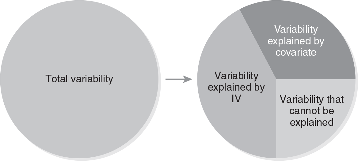
When we identify covariates that influence the dependent variable and carefully control for them in an ANCOVA, we achieve an important goal: we can explain the variability that we could not explain without the covariates. The unexplained variability is reduced, and the design allows us to more accurately examine the true effect of an independent variable. Similar to regression analysis, ANCOVA allows us to compute the percentage of variance attributed to the independent variable and the covariates—this process is called "partitioning." The partitioning of the variability is presented in Figure 13-1.

Partitioning of variability in analysis of covariance (ANCOVA).

A diagram shows the total variability in ANCOVA, analysis of covariance, partitioned into Variability explained by I V, Variability explained by covariate, and Variability that cannot be explained.

Assumptions

ANCOVA has all of the assumptions of ANOVA, plus two additional assumptions. These are (1) independence between the covariate and independent variable and (2) homogeneity of regression slope.

Independence between the covariate and independent variable makes sense as we try to reduce the variability that is not explained by the independent variable by explaining it with the covariates. If the covariate and the independent variable are dependent (overlapping), the variability that is computed will be difficult to interpret and it will be unclear whether it was explained by the independent variable.

Homogeneity of regression slope means that the relationship between the covariate and the dependent variable stays the same. For example, the health problem index should increase as the weight increases across all the workout groups.

Doing and Interpreting ANCOVA

First, we need to set up hypotheses. These look similar to those of ANOVA design, except the means are adjusted for the covariate:

H0: There is no difference among group means after adjusting for the covariate.

Ha: At least two group means differ after adjusting for the covariate.

or

H0: µ1 = µ2 = µ3 after adjusting for the covariate.

Ha: µj µk for some j and k after adjusting for the covariate.

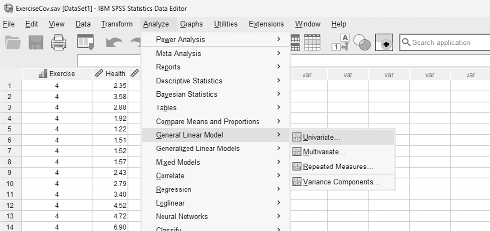
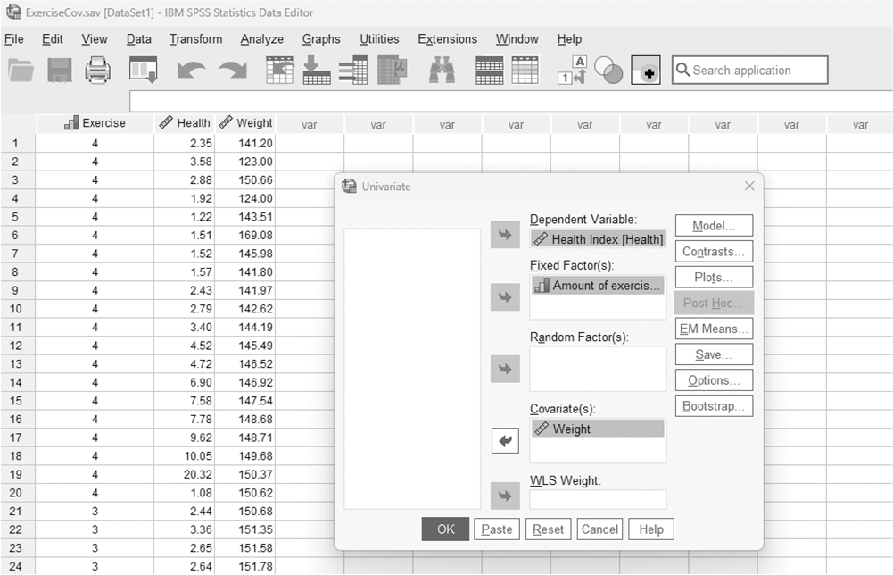
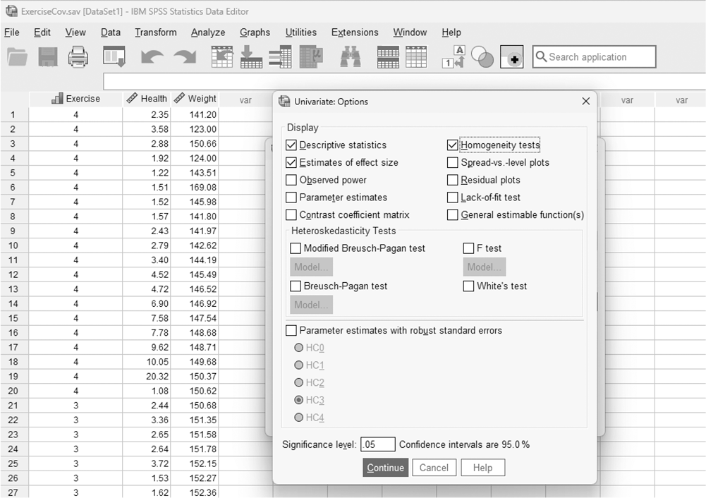
To conduct ANCOVA in IBM SPSS Statistics software (SPSS), you will open ExerciseCov.sav and go to Analyze > Generalized linear models > Univariate, as displayed in Figure 13-2. The data here are those we used in the multiple comparison example where the amount of exercise affected the health problem index. In the Univariate dialogue box, you will move the independent variable, Exercise, into "Fixed Factor(s)"; the dependent variable, Health, into "Dependent Variable"; and the covariate, Weight, into "Covariate(s)" by clicking the corresponding "arrow" buttons in the middle, as displayed in Figure 13-3. The box has six buttons, but only the commonly used buttons are discussed here. The "Contrasts" and "Post Hoc" buttons are used when further investigations are needed among more than two groups in the factor, with ANOVA results indicating substantial differences in group means, as discussed in the earlier section on planned contrasts and post hoc tests. The "Options" button gives us several choices that may help us interpret the ANCOVA results, which are presented in Figure 13-4. Please review the example output presented in Table 13-1.

Selecting ANCOVA under "General Linear Models" in SPSS.

A screenshot displays the SPSS menu with the Analyze tab open. The cursor highlights the General Linear Model submenu, and the option Univariate is visible within the dropdown list.

Reprint Courtesy of International Business Machines Corporation, © International Business Machines Corporation. "IBM SPSS Statistics software ("SPSS")". IBM®, the IBM logo, ibm.com, and SPSS are trademarks or registered trademarks of International Business Machines Corporation.

Defining variables in ANCOVA in SPSS.

A screenshot displays the Univariate dialog box in SPSS. Boxes labeled for dependent variables, fixed factors, and covariates appear at the center, with variable names listed on the left and selection buttons in between.

Reprint Courtesy of International Business Machines Corporation, © International Business Machines Corporation. "IBM SPSS Statistics software ("SPSS")". IBM®, the IBM logo, ibm.com, and SPSS are trademarks or registered trademarks of International Business Machines Corporation.

Useful options for ANCOVA in SPSS.

A screenshot displays an options dialog box in SPSS showing checkboxes for descriptive statistics, parameter estimates, and confidence intervals, with action buttons such as Continue and Cancel at the bottom.

Reprint Courtesy of International Business Machines Corporation, © International Business Machines Corporation. "IBM SPSS Statistics software ("SPSS")". IBM®, the IBM logo, ibm.com, and SPSS are trademarks or registered trademarks of International Business Machines Corporation. Courtesy of IBM SPSS Statistics.

Table 13-1 Example Output of ANCOVA in SPSS

Between-Subjects Factors

Value Label

N

Amount of Exercise

1

None

20

2

1 day per Week

20

3

3 days per Week

20

4

5 days per Week

20

Descriptive Statistics Dependent Variable: Health Index

Amount of Exercise

Mean

Std. Deviation

N

None

3.6031

6.38974

20

1 day per Week

5.1101

5.93392

20

3 days per Week

4.4770

3.50015

20

5 days per Week

4.8864

4.60177

20

Total

4.5191

5.16363

80

Levenes Test of Equality of Error Variancesa

Dependent Variable: Health Index

F

df1

df2

Sig.

.644

3

76

.589

Tests of Between-Subjects Effects Dependent Variable: Health Index

Source

Type III Sum of Squares

df

Mean Square

F

Sig.

Partial Eta-Squared

Corrected Model

169.937a

4

42.484

1.645

.172

.081

Intercept

112.647

1

112.647

4.363

.040

.055

Weight

143.437

1

143.437

5.555

.021

.069

Exercise

163.406

3

54.469

2.110

.106

.078

Error

1936.446

75

25.819

Total

3740.195

80

Corrected Total

2106.382

79

a R-Squared = .081 (Adjusted R-Squared = .032)

You will notice that the ANCOVA results table is similar to that of a one-way ANOVA, but there is an additional line representing the covariate—weight. The result indicates that weight substantially influences the health problem index with a small p-value of .007. However, you will find it interesting that the amount of exercise does not have a substantial effect on the health problem index with the covariate in the design. Do you remember that the amount of exercise made a substantial difference in the average health problem index value in one-way ANOVA? When we add the covariate, weight, to our analysis, we find that weight substantially influences the health problem index and cancels out the effect of exercise. If we had neglected to include the covariate of weight, we would have misinterpreted the influence of exercise on the health problem index.

Reporting ANCOVA

When reporting ANCOVA results, you should report the size of the F-statistics, along with associated degrees of freedom and associated p-value. For an effect size for ANCOVA, omega squared (ω2) can be calculated as it is with one-way ANOVA. Here, ω2 is only useful when the sample sizes for all groups are the same. Another type of effect size, partial eta squared (η2), is useful when sample sizes are not equal, and we can compute this in SPSS.

The following is a sample report from our example:

The covariate, weight, substantially influences this sample's health problem index, F (1, 75) = 5.55, p = .021. However, the amount of exercise per week did not influence the health problem index after controlling for the effect of weight, F (3, 75) = 2.11, p = .106, ω2 = .08.

Further group comparisons of the amount of exercise per week are not considered, as the overall test did not find substantial differences in the average health problem index.

Factorial Analysis of Variance (Anova)

One-way ANOVA allows us to examine the effect of one independent grouping variable on a dependent variable, which is why the design is called one-way ANOVA. However, an investigator often wants to examine the effect of more than one independent grouping variable on a dependent variable. For example, we may be interested in examining the effect of both the amount of exercise and the number of servings of soy milk per day on the health problem index. In this case, factorial ANOVA would be a good choice to examine the joint effect of the two independent variables. The design is called a two-way factorial ANOVA when there are two independent variables. With large sample sizes, there is the potential for three-, four-, and five-way factorial ANOVA, but this text will only consider two-way factorial ANOVA. In factorial ANOVA, each level of each factor (independent variable) is crossed with each level of another factor so that we can examine the interaction effect between factors/independent variables. In our present example, we examine the mean differences between one serving of soy milk per day and no exercise per week, one serving of soy milk and 1 day of exercise per week, one serving of soy milk and 3 days of exercise per week, then two servings of soy milk and 1 day of exercise per week, and so on (you get the idea). (Refer to Table 13-2.) An interaction effect is present when the differences explained by one factor depend upon those by the other factor.

Table 13-2 Example Permutations of a Two-Way Factorial ANOVA

Factor A (Amount of Exercise)

None (A1)

1 Day per Week (A2)

3 Days per Week (A3)

5 Days per Week (A4)

Factor B (servings of soy milk)

None (B1)

A1B1

A2B1

A3B1

A4B1

1 cup of milk (B2)

A1B2

A2B2

A3B2

A4B2

2 cups of milk (B3)

A1B3

A2B3

A3B3

A4B3

3 cups of milk (B4)

A1B4

A2B4

A3B4

A4B4

Doing and Interpreting Factorial ANOVA

First, we need to set up hypotheses. Because we have two independent factors, we need hypotheses for each of the factors and another for the interaction effects between the two factors:

H01: There is no difference among group means in Factor A.

Ha1: At least two group means in Factor A differ.

or

H01: µ1 = µ2 = µ3

Ha1: µj µk for some j and k

H02: There is no difference among group means in Factor B.

Ha2: At least two group means in Factor B differ.

H03: There is no interaction effect between Factor A and B.

Ha3: There is an interaction effect between Factor A and B.

The test statistic for each hypothesis in factorial ANOVA can be found by the same equation:

Formula reads: F equals Differences between groups over Differences within groups.

where differences between groups are divided into three components: (1) differences between groups explained by Factor A, (2) differences between groups explained by Factor B, and (3) differences between groups explained by the interaction of Factors A and B. We evaluate the associated p-value with this statistic and make a decision (i.e., reject the null hypothesis when the p-value associated with the computed statistic is small or not reject when the p-value associated with the computed statistic is large). Of course, we will support this statistical result with a measure of effect size and a corresponding interval estimate (i.e., confidence interval) as a measure of importance.

Results are reported as the main effect and interaction effect. The main effect is the group difference between each of the independent (grouping) variables on the dependent variables. The interaction effect reflects the interaction of grouping variables on the dependent variables. Be sure to look at the interaction effect first, as the main effect of an independent variable compares the means of its groups without considering another independent variable—that is, the results of the main effect cannot be trusted when the effect of one factor is associated with the effect of another factor. In that case, you need to conduct a simple effect analysis, which looks at the effect of one variable at each level of the other variable to determine if the results of a given main effect happen at all levels of the other variable. In contrast, the main effect results can be interpreted as when a substantial interaction effect does not exist.

To conduct a two-way factorial ANOVA in Excel, you will open ExerciseFA.xlsx and note that the data should be formatted differently, as presented in Figure 13-5. Go to Data > Data Analysis, as presented in Figure 13-6, and choose "ANOVA: Two-Factor With Replication" (Figure 13-7), as we have four groups of exercise, and individuals within each group are doing more than one thing (i.e., drinking four different amounts of milk). In the "ANOVA: Two-Factor With Replication" dialogue box, you will provide A1:E21 as the Input Range and insert "5" as Rows per sample (Figure 13-8). Clicking "OK" will produce the requested regression analysis output. The example output is presented in Figure 13-9.

Formatting the data for analysis in Excel.
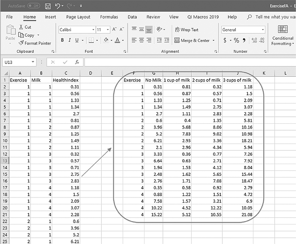
An Excel screenshot shows the formatting of data of conduct a two-way factorial ANOVA.

There are three columns of numerical data: Exercise, Milk, and Healthindex. The values of Milk range between 1 and 4, with 1 indicating No milk, 2 indicating 1 cup of milk, 3 indicating 2 cups of milk, and 4 indicating 3 cups of milk. An arrow points to another table with columns, Exercise, No milk, 1 cup of milk, 2 cups of milk, 3 cups of milk, with values from the column Milk transferred to Exercise, and the other columns containing numerical data with decimals.

Courtesy of Microsoft Excel © Microsoft 2020.

Finding Data Analysis ToolPak in Excel.
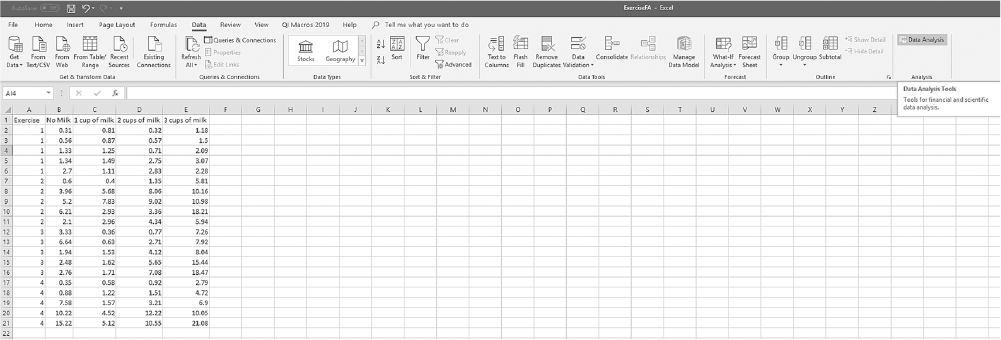
An Excel screenshot shows the Data Analysis ToolPak add-in, in the Analysis group under Data menu.

Courtesy of Microsoft Excel © Microsoft 2020.

Selecting "ANOVA: Two-Factor With Replication" in Excel.
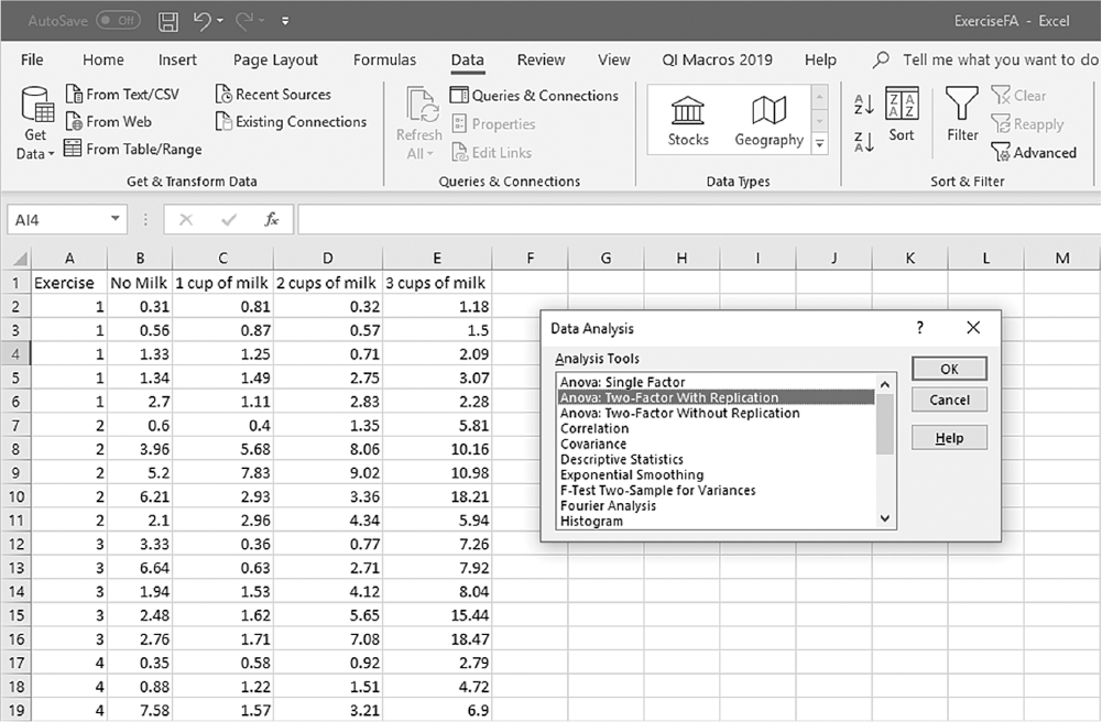
An Excel screenshot shows selection of the option, ANOVA: two-factor with replication, within the Data Analysis Tools. The worksheet lists the five columns, Exercise, No milk, 1 cup of milk, 2 cups of milk, 3 cups of milk, with numerical data.

Courtesy of Microsoft Excel © Microsoft 2020.

Defining data ranges and selecting options for "ANOVA: Two-Factor With Replication" in Excel.
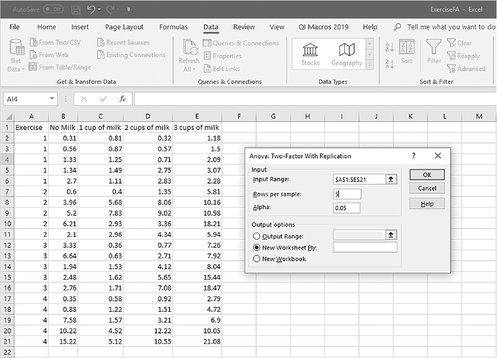
An Excel screenshot shows the ANOVA: two-factor with replication dialog box with fields to define data. The worksheet lists the five columns, Exercise, No milk, 1 cup of milk, 2 cups of milk, 3 cups of milk, with numerical data.

The dialog box has two textboxes. The first textbox with heading, Input, consists of a drop-down list, input range; the entry field Rows per sample has the value 5 entered in it. The second textbox with heading, Output options, consists of a drop-down list, output range; new worksheet ply which is checked; and new worksheet. The buttons, O k, Cancel, and Help, are on the right of the dialog box.

Courtesy of Microsoft Excel © Microsoft 2020.

Example output for "ANOVA: Two-Factor With Replication" in Excel.
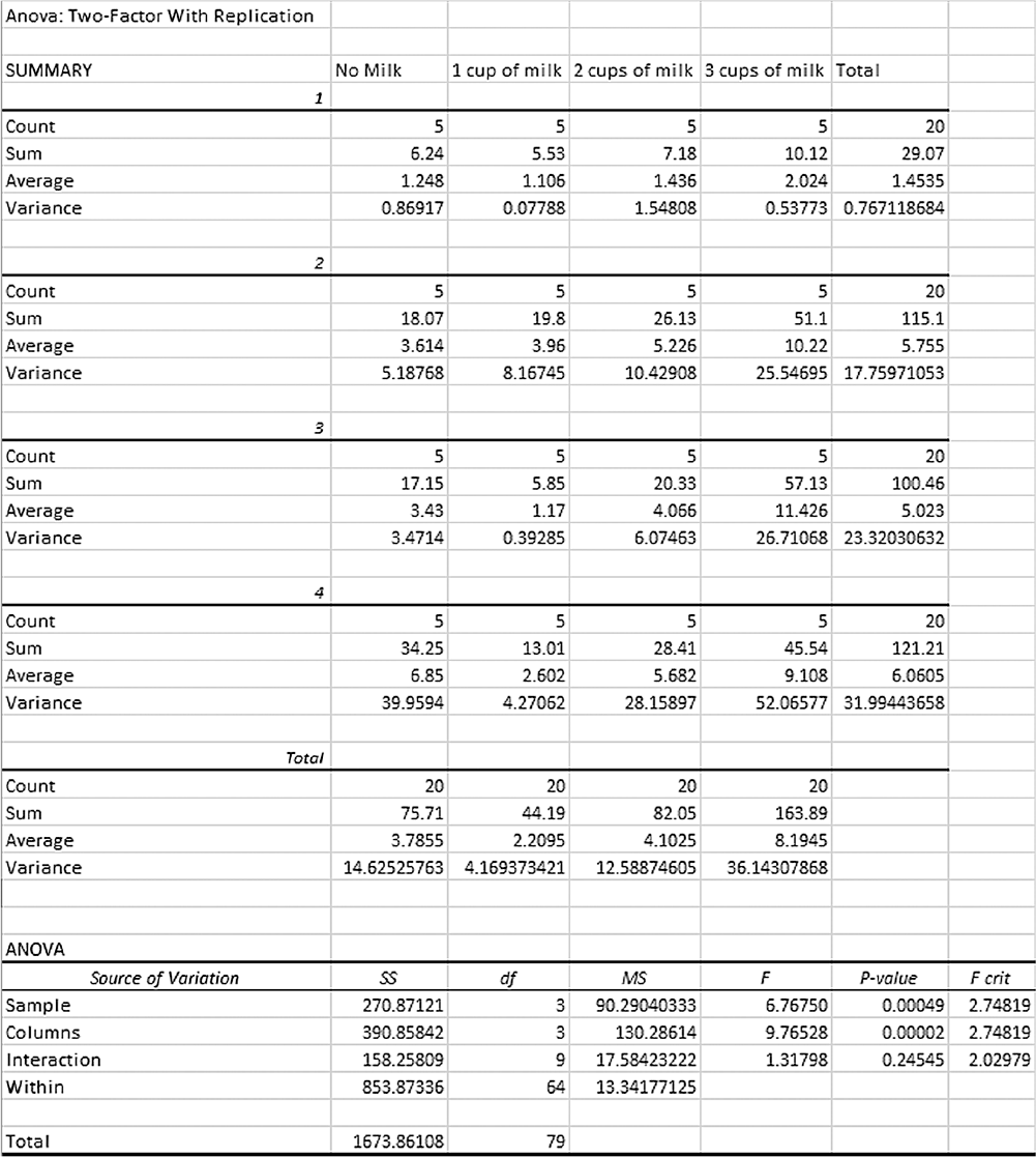
An Excel screenshot shows an output of the ANOVA: Two-factor with replication.

A table is divided into six sections, with the first five sections consisting of five columns: Exercise, No milk, 1 cup of milk, 2 cups of milk, 3 cups of milk, and Total. The first section is Exercise 1, and the row entries are as follows. Row 1: Count, 5, 5, 5, 5, 20. Row 2: Sum, 6.24, 5.53, 7.18, 10.12, 29.07. Row 3: Average, 1.248, 1.106, 1.436, 2.024, 1.4535. Row 4: Variance, 0.86917, 0.07788, 1.54808, 0.53773, 0.767118684. The second section is Exercise 2, and the row entries are as follows. Row 1: Count, 5, 5, 5, 5, 20. Row 2: Sum, 18.07, 19.8, 26.13, 51.1, 115.1. Row 3: Average, 3.614, 3.96, 5.226, 10.22, 5.755. Row 4: Variance, 5.18768, 8.16745, 10.42908, 25.54695, 17.75971053. The third section is Exercise 3, and the row entries are as follows. Row 1: Count, 5, 5, 5, 5, 20. Row 2: Sum, 17.15, 5.85, 20.33, 57.13, 100.46. Row 3: Average, 3.43, 1.17, 4.066, 11.426, 5.023. Variance: 3.4714, 0.39285, 6.07463, 26.71068, 23.32030632. The fourth section is Exercise 4, and the row entries are as follows. Row 1: Count, 5, 5, 5, 5, 20. Row 2: Sum, 34.25, 13.01, 28.41, 45.54, 121.21. Row 3: Average, 6.85, 2.602, 5.682, 9.108, 6.0605. Row 4: Variance, 39.9594, 4.27062, 28.15897, 52, 06577, 31.99443658. The fifth section is Total, and the row entries are as follows. Row 1: Count, 20, 20, 20, 20, no data. Row 2: Sum, 75.71, 44.19, 82.05, 163.89, no data. Row 3: Average, 3.7855, 2.2095, 4.1025, 8.1945, no data. Row 4: Variance, 14.62525763, 4.169373421, 12.58874605, 36.14307868, no data. The last section, titled ANOVA, consists of seven columns: Source of Variation, S S, d f, M S, F, p-value, F crit. The row entries are as follows. Row 1: Sample, 270.87121, 90.29040333, 6.76750, 0.00049, 2.76819. Row 2: Columns, 390.85842, 3, 130.28614, 9.76528, 2.74819. Row 3: Interaction, 158.25809, 9, 17.58423222, 1.31798, 0.24545, 2.02979. Row 4: Within, 853.87335, 64, 13.34177125, no data, no data, no data. Row 5: Total, 1673.86108, 79, no data, no data, no data, no data.

Courtesy of Microsoft Excel © Microsoft 2020.

To conduct a two-way factorial ANOVA in SPSS, you will open ExerciseFA.sav and go to Analyze > General Linear Model > Univariate, as presented in Figure 13-10. The variables presented in Figure 13-11 represent the amount of exercise and the number of servings of soy milk consumed per day as independent variables and the health problem index as a dependent variable. In the Univariate dialogue box, you will move the independent variables into "Fixed Factor(s)" and a dependent variable into "Dependent Variable" by clicking the corresponding arrow buttons in the middle, as presented in Figure 13-11. The button has six buttons, but only the commonly used buttons are discussed here. The "Contrasts" and "Post Hoc" buttons are used when further investigations are needed among more than two groups in the factor with an overall group difference from ANOVA results, as discussed in the earlier section on planned contrasts and post hoc tests. The "Plots" button can help us interpret the interaction effect visually and can be created, as presented in Figure 13-12. The "Options" button gives us several choices that may help us interpret the results of factorial ANOVA; these are presented in Figure 13-13. Clicking "OK" will produce the requested factorial ANOVA analysis output. An example output is presented in Table 13-3.

Selecting factorial ANOVA under "General Linear Model" in SPSS.
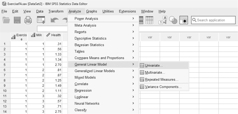
A screenshot displays the SPSS interface with the Analyze menu open. The cursor highlights the General Linear Model submenu, and the option Univariate appears in the dropdown list.

Reprint Courtesy of International Business Machines Corporation, © International Business Machines Corporation. "IBM SPSS Statistics software ("SPSS")". IBM®, the IBM logo, ibm.com, and SPSS are trademarks or registered trademarks of International Business Machines Corporation.

Defining variables in factorial ANOVA in SPSS.
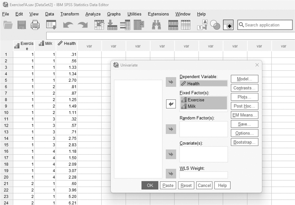
A screenshot displays the Univariate dialog box in SPSS. Sections for dependent variables and fixed factors are shown, with variable names listed on the left and arrow buttons used to assign variables to each field.

Reprint Courtesy of International Business Machines Corporation, © International Business Machines Corporation. "IBM SPSS Statistics software ("SPSS")". IBM®, the IBM logo, ibm.com, and SPSS are trademarks or registered trademarks of International Business Machines Corporation.

Creating an interaction plot in factorial ANOVA in SPSS.
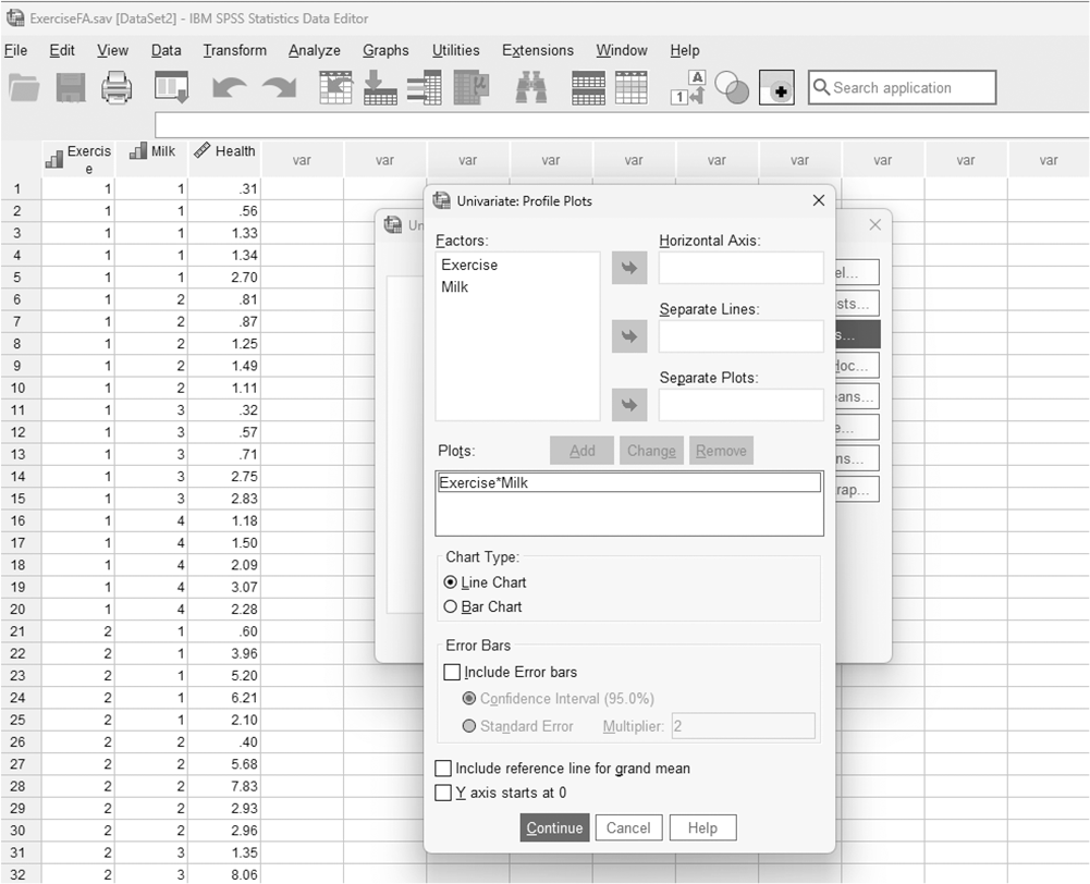
A screenshot displays the SPSS dialog box for interaction plots. Options to select factors for the horizontal axis and separate lines are visible, with buttons labeled Add, Remove, and Continue.

Reprint Courtesy of International Business Machines Corporation, © International Business Machines Corporation. "IBM SPSS Statistics software ("SPSS")". IBM®, the IBM logo, ibm.com, and SPSS are trademarks or registered trademarks of International Business Machines Corporation.

Useful options for factorial ANOVA in SPSS.
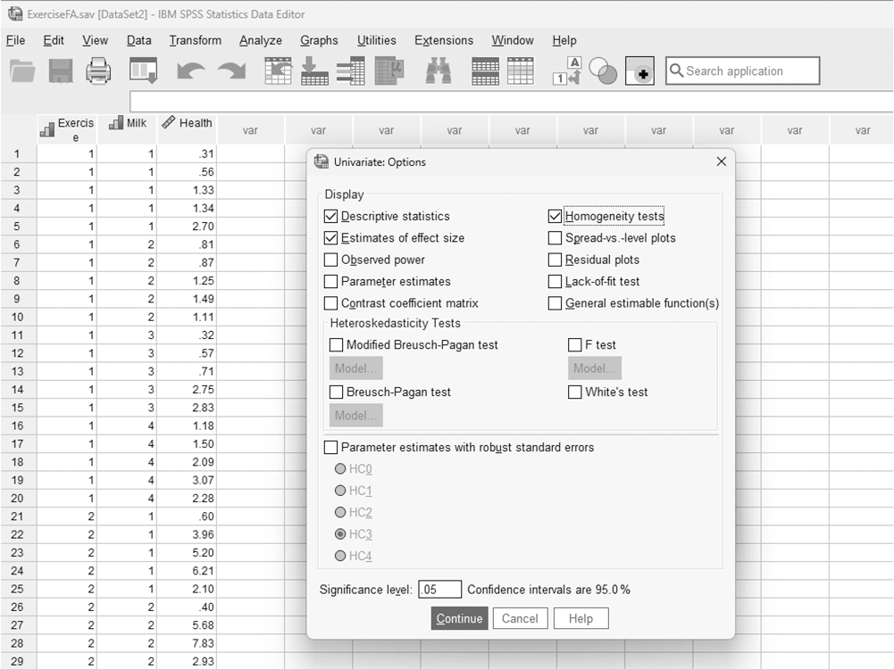
A screenshot displays the SPSS options window containing checkboxes for descriptive statistics, estimates of effect size, and homogeneity tests, with Continue and Cancel buttons at the bottom.

Reprint Courtesy of International Business Machines Corporation, © International Business Machines Corporation. "IBM SPSS Statistics software ("SPSS")". IBM®, the IBM logo, ibm.com, and SPSS are trademarks or registered trademarks of International Business Machines Corporation.

Table 13-3 Example Output of Factorial ANOVA in SPSS

Between-Subjects Factors

Value Label

N

Exercise

1

None

20

2

1 day per week

20

3

3 days per week

20

4

5 days per week

20

Milk

1

None

20

2

1 cup of milk

20

3

2 cups of milk

20

4

3 cups of milk

20

Levenes Test of Equality of Error Variancesa,b

Levene Statistic

df1

df2

Sig.

Health

Based on mean

4.508

15

64

<.001

Based on median

1.795

15

64

.055

Based on median and with adjusted df

1.795

15

23.904

.098

Based on trimmed mean

4.350

15

64

<.001

Tests the null hypothesis that the error variance of the dependent variable is equal across groups.

a. Dependent variable: Health

b. Design: Intercept + Exercise + Milk + Exercise * Milk

Tests of Between-Subjects Effects

Dependent Variable: Health

Source

Type III Sum of Squares

df

Mean Square

F

Sig.

Partial Eta- Squared

Corrected model

819.988a

15

54.666

4.097

<.001

.490

Intercept

1672.986

1

1672.986

125.395

<.001

.662

Exercise

270.871

3

90.290

6.767

<.001

.241

Milk

390.858

3

130.286

9.765

<.001

.314

Exercise *Milk

158.258

9

17.584

1.318

.245

.156

Error

853.873

64

13.342

Total

3346.847

80

Corrected total

1673.861

79

a. R-Squared = .490 (Adjusted R-Squared = .370)

Descriptive Statistics Dependent Variable: Health

Exercise

Milk

Mean

Std. Deviation

N

None

None

1.2480

.93229

5

1 cup of milk

1.1060

.27907

5

2 cups of milk

1.4360

1.24422

5

3 cups of milk

2.0240

.73330

5

Total

1.4535

.87585

20

1 day per week

None

3.6140

2.27765

5

1 cup of milk

3.9600

2.85788

5

2 cups of milk

5.2260

3.22941

5

3 cups of milk

10.2200

5.05440

5

Total

5.7550

4.21423

20

3 days per week

None

3.4300

1.86317

5

1 cup of milk

1.1700

.62678

5

2 cups of milk

4.0660

2.46468

5

3 cups of milk

11.4260

5.16824

5

Total

5.0230

4.82911

20

5 days per week

None

6.8500

6.32134

5

1 cup of milk

2.6020

2.06655

5

2 cups of milk

5.6820

5.30650

5

3 cups of milk

9.1080

7.21566

5

Total

6.0605

5.65636

20

Total

None

3.7855

3.82430

20

1 cup of milk

2.2095

2.04190

20

2 cups of milk

4.1025

3.54806

20

3 cups of milk

8.1945

6.01191

20

Total

4.5730

4.60305

80

You will notice that Levene's test for the assumption of homogeneity of variance is violated, but ANOVA designs tend to be robust when the sample sizes across the groups are the same. From the interaction plot (Profile Plots), we can observe that the lines look relatively parallel to each other. When the lines in the interaction plot are parallel, we say there is no interaction effect between the two factors; if the lines cross, there is an interaction effect. In this case, there is no interaction between servings of soy milk per day and the level of exercise.

In the "Test of Between-Subjects Effects" table, the two main factors (exercise and amount of soy milk consumed) were found to have substantial effects on the health index, but the interaction between them was not substantial. Because one factor is not dependent upon the other factor from its nonsubstantial effect (i.e., one factor does not work with the other factor to make changes on the means of the dependent variable), the main effects can be interpreted as they are. Both the amount of exercise and the amount of milk consumed per day substantially affect the health problem index, but we still do not know how the groups (levels of exercise and amount of milk consumed) differ. Therefore, Bonferroni tests on both factors should be done as post hoc tests; these results are presented in Table 13-4. The output indicates that people who exercise 0 days per week have a substantially lower health index than those who exercise at least 1 day per week. We can also notice that people who drank 3 cups of soy milk have a substantially higher health index than those who drank less than 3 cups of soy milk.

Table 13-4 Post Hoc Test Results of Factorial ANOVA in SPSS

Exercise Multiple Comparisons Dependent Variable: Health Bonferroni

(I) Exercise

(J) Exercise

Mean Difference (I-J)

Std. Error

Sig.

95% Confidence Interval

Lower Bound

Upper Bound

None

1 day per Week

μ4.3015*

1.15507

0.002

μ7.4464

μ1.1566

3 days per Week

μ3.5695*

1.15507

0.018

μ6.7144

-0.4264

5 days per Week

μ4.6070*

1.15507

0.001

μ7.7519

μ1.4621

1 day per Week

None

4.3015*

1.15507

0.002

1.1566

7.4464

3 days per Week

.7320

1.15507

1.000

μ2.4129

3.8769

5 days per Week

μ.3055

1.15507

1.000

μ3.4504

2.8394

3 days per week

None

3.5695*

1.15507

0.018

.4246

6.7144

1 day per Week

μ.7320

1.15507

1.000

μ3.8769

2.4129

5 days per Week

μ1.0375

1.15507

1.000

μ4.1824

2.1074

5 days per Week

None

4.6070*

1.15507

0.001

1.4621

7.7519

1 day per Week

0.3055

1.15507

1.000

μ2.8394

3.4504

3 days per Week

1.0375

1.15507

1.000

μ2.1074

4.1824

Based on observed means.

The error term is Mean Square(Error) = 13.342.

*The mean difference is significant at the .05 level.

Milk Multiple Comparisons Dependent Variable: Health Bonferroni

(I) Milk

(J) Milk

Mean Difference (I-J)

Std.Error

Sig.

95% Confidence Interval

Lower Bound

Upper Bound

None

1 cup of milk

1.5760

1.15507

1.000

μ1.5689

4.7209

2 cups of milk

μ.3170

1.15507

1.000

μ3.4619

2.82 79

3 cups of milk

μ4.4090*

1.15507

.002

μ7.5539

μ1.2641

1 cup of milk

None

μ1.5760

1.15507

1.000

μ4.7209

1.5689

2 cups of milk

μ1.8930

1.15507

.637

μ5.0379

1.2519

3 cups of milk

μ5.9850*

1.15507

<.001

μ9.1299

μ2.8401

2 cups of milk

None

.3170

1.15507

1.000

μ2.8279

3.4619

1 cup of milk

1.8930

1.15507

.637

μ1.2519

5.0379

3 cups of milk

μ4.0920*

1.15507

.004

μ7.2369

μ.94 71

3 cups of milk

None

4.4090*

1.15507

.002

1.2641

7.5539

1 cup of milk

5.9850*

1.15507

<.001

2.8401

9.1299

2 cups of milk

4.0920*

1.15507

.004

.9471

7.2369

Based on observed means.

The error term is Mean Square (Error) = 13.342.

*The mean difference is significant at the .05 level.

Reporting Two-Way Factorial ANOVA

Reporting two-way factorial ANOVA results is similar to that in one-way ANOVA. You should report the size of F-statistics along with associated degrees of freedom and associated p-value for both the main effect and interaction effect. The computation of effect size for any factorial ANOVA design is more complicated and cumbersome than for one-way ANOVA, but we can obtain and report estimates of effect size, partial η2, as presented in Figure 13-13. We recommend that you compute and interpret other types of effect size in consultation with a statistician.

The following is a sample report from our example:

  • There was no interaction effect between the amount of exercise per week and the number of servings of soy milk per day on the health index, F (9, 64) = 1.32, p = .245, η2 = .156.

  • There was a substantial effect of the amount of exercise per week on the health index, F (3, 64) = 6.77, p< .001, η2 = .241. The Bonferroni test revealed that the group that did not exercise had a substantially lower health index than those who exercised 1 day per week (p =.002, 95% CI [-7.45, -1.16]), those who exercised 3 days per week (p = .018, 95% CI [-6.71, -0.43]), and those who exercised 5 days per week (p = .001, 95% CI [-7.75, -1.46]).

  • There was also a substantial effect of the number of servings of soy milk drunk per day on health index: F (3, 64) = 9.77, p = .001, η2 =.314. The Bonferroni test revealed that the group who drank 3 cups of soy milk per day had a substantially higher health index than those who drank no milk (p = .002, 95% CI [1.26, 7.55]), those who drank 1 cup of milk (p = .000, 95% CI [2.84, 9.13]), and those who drank 2 cups of milk (p = .004, 95% CI [0.94, 7.24]).

Repeated Measures Anova

Introduction

Until now, we have discussed ANOVA designs where several independent group means are compared. However, there are situations where three or more group means come from the same group of participants, similar to what we discussed in dependent samples t-test. Repeated measures ANOVA is an extended design of the dependent samples t-test where there are more than two measurements in the same group of participants. Recall that repeated measures design can take two different forms. The first is when the same variable is measured multiple times with the same group of participants to consider changes over time; and the second is when multiple treatments are given to the same group of participants to compare responses to each treatment. Repeated measures ANOVA can also be used when sample members are matched based on some important characteristics. For example, male and female nursing home residents may be matched when a researcher is interested in examining the level of sleep disturbance since they reside in the same environment.

Repeated measures ANOVA design provides the following advantages:

  • It is suitable when some variables are to be measured repeatedly over time (i.e., longitudinal design).

  • It is an economical design compared with independent sample group comparison because the required sample size is smaller than when you have more than one group.

  • Because it analyzes only one group, the variability is lower than in a multigroup design, and therefore the validity of results will be higher.

However, there are disadvantages:

  • Repeated measurements may not be possible because of dropout, death, and so on.

  • There may be a maturation effect where the subjects change over the course of the study.

  • There may be other effects that reduce the validity of results, such as subjects' scores converging on the average with multiple measurements.

Assumptions

Repeated measures ANOVA assumptions are similar to those required by one-way ANOVA, such as normality and homogeneity of variance. Similar to other ANOVA designs, repeated measures ANOVA is robust to the violation of the normality and homogeneity of variance, especially when group sample sizes are the same. Note that the assumption of homogeneity of variance only applies when groups are compared along with repeated measures. However, the last assumption of independence is automatically violated because the measurements come from the same participant group. Instead, the assumption of relations between/ among repeated measures, the assumption of sphericity, is added and should be tested. The assumption of sphericity means that the variances of the differences, as well as the correlations among the repeated measures, are all equal.

Doing and Interpreting Repeated Measures ANOVA

First, we need to set up hypotheses:

H0: There is no difference among repeated measure means.

H1: At least two repeated measure means differ.

or

H01: µ1 = µ2 = µ3

Ha1: µj µk for some j and k.

The test statistic each hypothesis in repeated measures ANOVA can be found by the following equation:

Formula reads: F equals Differences between time measurements over Differences within each measurement.

Once the statistic is computed, we evaluate whether the associated p-value is small enough to rule out chance; in other words, is the p-value small or large enough to indicate evidence for an effect? As discussed earlier, it is important to support the p-value with a measure of effect size, along with a corresponding interval estimate (i.e., confidence interval), as a measure of importance.

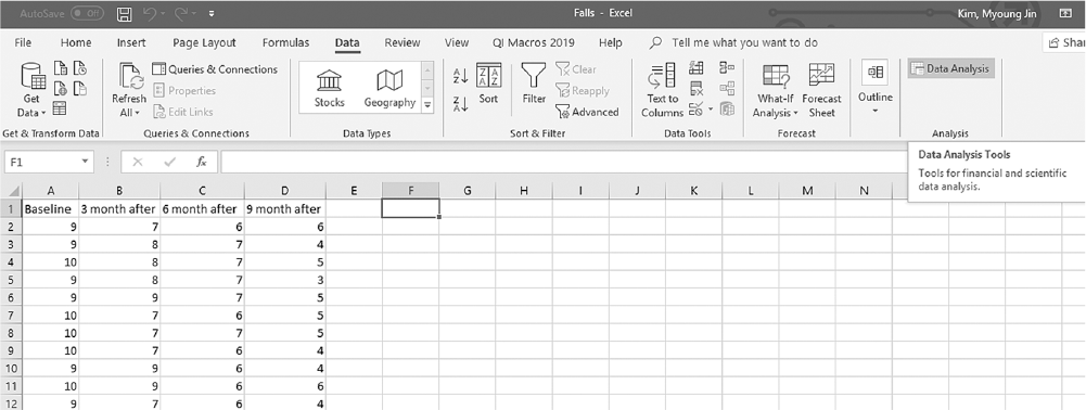
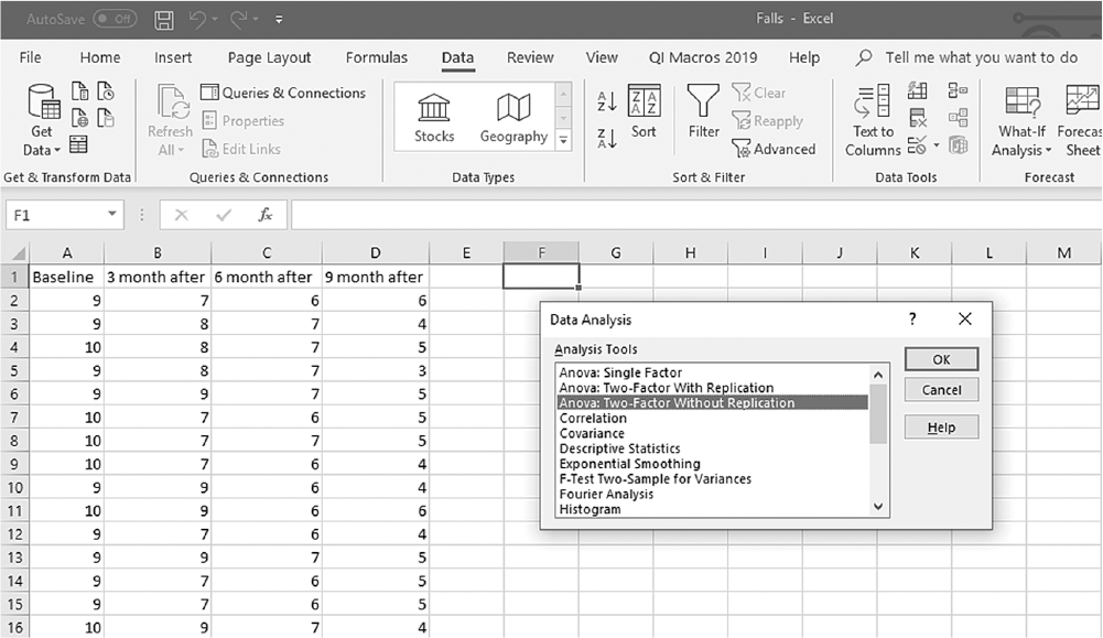
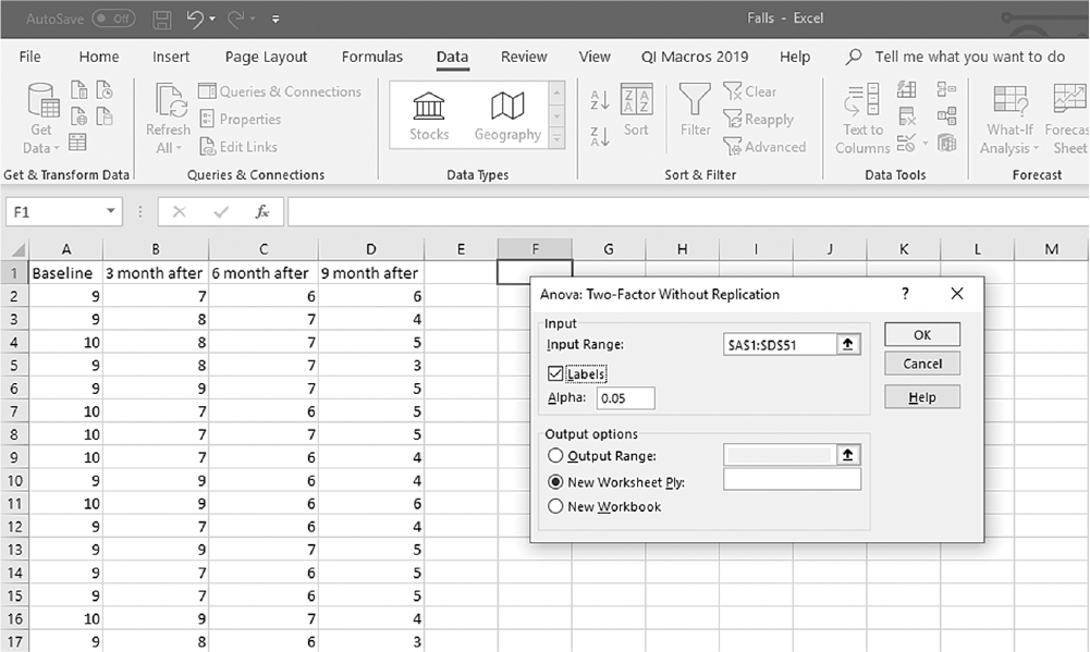
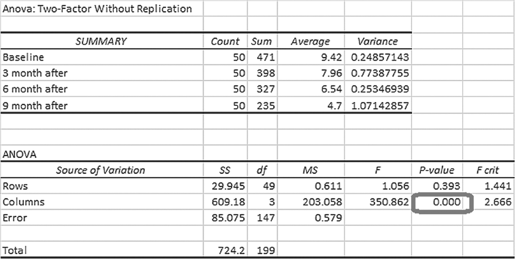
To conduct a repeated measures ANOVA in Excel, you will open Falls.xlsx (the data presented in the figure are the number of falls across four times: baseline, 3 months after, 6 months after, and 9 months after implementing a newly developed fall prevention intervention) and go to Data > Data Analysis, as presented in Figure 13-14. In the Data Analysis window, you will note that "ANOVA: Two-Factor Without Replication" is on the list (Figure 13-15), as only one group is doing more than one thing (i.e., getting measured on four different occasions). In the "ANOVA: Two-Factor Without Replication" dialogue box, you will provide A1:D51 as Input Range with "Labels" checked (Figure 13-16). Clicking "OK" will then produce the output of the requested regression analysis. The example output is presented in Figure 13-17.

Finding the Data Analysis ToolPak in Excel.

An Excel screenshot shows the Data Analysis ToolPak add-in, in the Analysis group under Data menu.

Courtesy of Microsoft Excel © Microsoft 2020.

Selecting "ANOVA: Two-Factor Without Replication" in Excel.

An Excel screenshot shows selection of the option, ANOVA: two-factor without replication, within the Data Analysis Tools. The worksheet lists the four columns, baseline, 3 month after, 6 month after, and 9 month after, with numerical data.

Courtesy of Microsoft Excel © Microsoft 2020.

Defining data ranges and selecting options for "ANOVA: Two-Factor Without Replication" in Excel.

An Excel screenshot shows the ANOVA: two-factor without replication dialog box with fields to define data. The worksheet lists the four columns, baseline, 3 month after, 6 month after, and 9 month after, with numerical data.

The dialog box has two textboxes. The first textbox with heading, Input, consists of a drop-down list, input range; Labels is checked. The second textbox with heading, Output options, consists of a drop-down list, output range; new worksheet ply which is checked; and new worksheet. The buttons, O k, Cancel, and Help, are on the right of the dialog box.

Courtesy of Microsoft Excel © Microsoft 2020.

Example output for "ANOVA: Two-Factor Without Replication" in Excel.

An Excel screenshot displaying the output for ANOVA: Two-factor without replication.

The first table has five columns: Summary, Count, Sum, Average, and Variance. The row entries are as follows. Row 1: Baseline, 50, 471, 9.42, 0.24857143. Row 2: 3 month after, 50, 398, 7.96, 0.77387755. Row 3: 6 month after, 50, 327, 6.54, 0.25346939. Row 4: 9 month after, 50, 235, 4.7, 1.07142857. The second table, titled ANOVA, has seven columns: Source of variation, S S, d f, M S, F, p-value, and F crit. The row entries are as follows. Row 1: Rows, 29.945, 49, 0.611, 1.056, 0.393, 1.441. Row 2: Columns, 609.18, 3, 203.058, 350.862, 0.000, 2.666. Row 3: Error, 85.075, 147, 0.579, no data, no data, no data. Row 4: Total, 724.2, 199, no data, no data, no data, no data. The value, 0.000, is highlighted.

Courtesy of Microsoft Excel © Microsoft 2020.

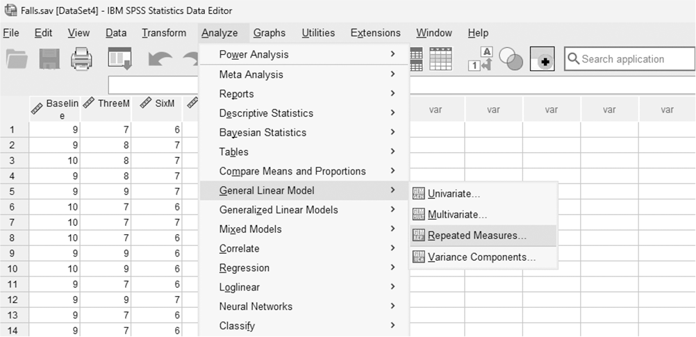
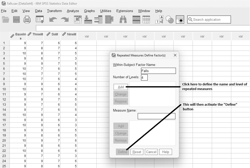
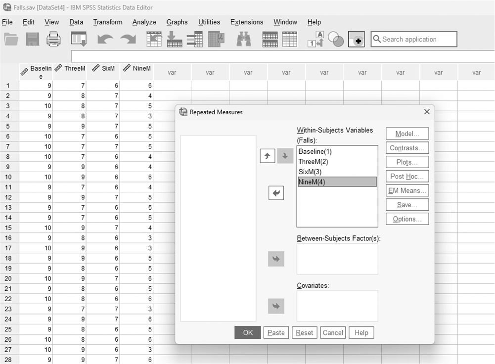
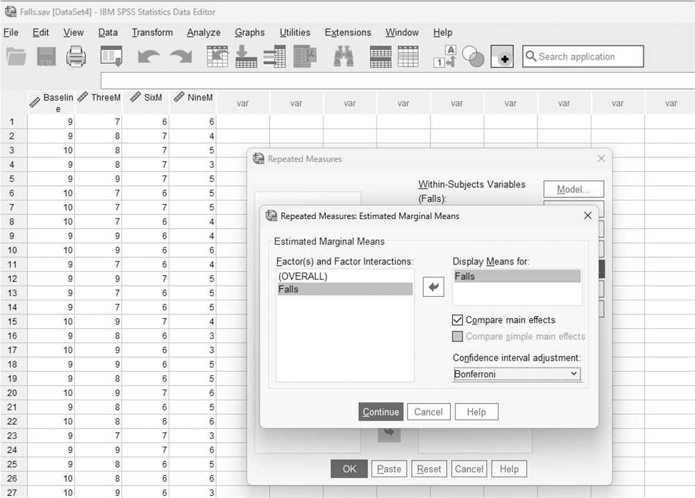
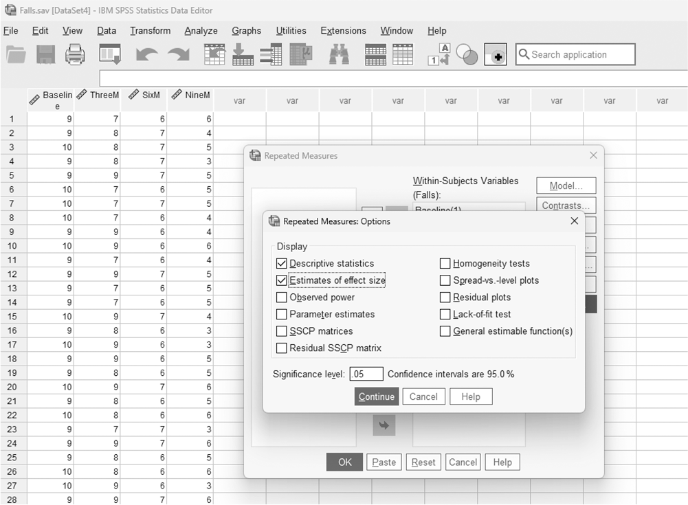
To conduct a repeated measures ANOVA in SPSS, you will open Falls.sav and go to Analyze > General Linear Model > Repeated Measures, as presented in Figure 13-18. This will bring up the Repeated Measures Define Factor(s) dialogue box; here, the name of the within-subject factor and the number of repeated measures should be identified as presented in Figure 13-19. In this example, the data are the number of falls across four times: baseline, 3 months after, 6 months after, and 9 months after implementing a newly developed fall prevention intervention. Type "Falls" for name and "4" for level since there are four measurements, and then click "Define." In the Repeated Measures dialogue box, you will notice that four levels with question marks are already displayed under "Within-Subjects Variable(s)," so now you need to instruct SPSS what those levels are. Move the corresponding levels starting with the first measurement, in this case "baseline," until every level is moved in order by clicking an arrow button in the middle, as presented in Figure 13-20. The box has six buttons, but only the commonly used buttons are discussed here. The "Contrasts" and "Post Hoc" buttons are used when further investigations are needed among more than two groups in the factor with an overall group difference from ANOVA results, as discussed earlier. However, we have only one group in this example, so they are skipped here. However, the overall significance test in repeated measures ANOVA only indicates a substantial difference between time measurements. It does not indicate which measurements differ from the other measurements. The "EM Means" button provides a basic set of the post hoc tests in case the overall test indicates that there is a difference among the repeated measures (Figure 13-21), and the "Options" button provides several options that may help us interpret the results of repeated measures ANOVA (Figure 13-22). Clicking "OK" will then produce the output of the requested analysis. Here, you will notice Bonferroni pairwise comparison results that will help us determine which measurements actually differ from the other measurements. An example output is presented in Table 13-5.

Selecting repeated measures ANOVA under "General Linear Model" in SPSS.

A screenshot displays the SPSS interface with the Analyze menu open. The cursor points to the General Linear Model submenu, and the option Repeated Measures is visible in the dropdown list.

Reprint Courtesy of International Business Machines Corporation, © International Business Machines Corporation. "IBM SPSS Statistics software ("SPSS")". IBM®, the IBM logo, ibm.com, and SPSS are trademarks or registered trademarks of International Business Machines Corporation.

Defining the name and level of repeated measures in repeated measures ANOVA in SPSS.

A screenshot displays the SPSS dialog box for defining repeated measures. Fields for entering the within-subject factor name and number of levels are visible, with Define and Cancel buttons below.

Reprint Courtesy of International Business Machines Corporation, © International Business Machines Corporation. "IBM SPSS Statistics software ("SPSS")". IBM®, the IBM logo, ibm.com, and SPSS are trademarks or registered trademarks of International Business Machines Corporation.

Defining variables in repeated measures ANOVA in SPSS.

A screenshot displays the SPSS repeated measures dialog box showing boxes for within-subject variables and dependent variables. Variable names appear on the left, and arrow buttons are used to assign them.

Reprint Courtesy of International Business Machines Corporation, © International Business Machines Corporation. "IBM SPSS Statistics software ("SPSS")". IBM®, the IBM logo, ibm.com, and SPSS are trademarks or registered trademarks of International Business Machines Corporation.

Post hoc tests for repeated measures ANOVA in SPSS.

A screenshot displays the SPSS post hoc dialog box with a list of variables on the left and available test options such as Bonferroni and Tukey on the right, along with Continue and Cancel buttons at the bottom.

Reprint Courtesy of International Business Machines Corporation, © International Business Machines Corporation. "IBM SPSS Statistics software ("SPSS")". IBM®, the IBM logo, ibm.com, and SPSS are trademarks or registered trademarks of International Business Machines Corporation.

Useful options for repeated measures ANOVA in SPSS.

A screenshot displays the SPSS options window showing checkboxes for descriptive statistics, estimates of effect size, and homogeneity tests, with Continue and Cancel buttons positioned at the bottom.

Reprint Courtesy of International Business Machines Corporation, © International Business Machines Corporation. "IBM SPSS Statistics software ("SPSS")". IBM®, the IBM logo, ibm.com, and SPSS are trademarks or registered trademarks of International Business Machines Corporation.

Table 13-5 Example Output of Repeated Measures ANOVA in SPSS

WithinμSubjects Factors Measure: MEASURE_1

Falls

Dependent Variable

1

Baseline

2

ThreeM

3

SixM

4

NineM

Descriptive Statistics

Mean

Std. Deviation

N

Number of falls at Baseline

9.42

.499

50

Number of falls after 3 months

7.96

.880

50

Number of falls after 6 months

6.54

.503

50

Number of falls after 9 months

4.70

1.035

50

Tests of Within-Subjects Effects Measure: MEASUR E_1

Source

Type III Sum of Squares

df

Mean Square

F

Sig.

Partial Eta-Squared

Falls

Sphericity Assumed

609.175

3

203.058

350.862

<.001

.877

Greenhouse μ Geisser

609.175

2.329

261.578

350.862

<.001

.877

Huynh μFeldt

609.175

2.452

248.430

350.862

<.001

.877

Lower bound

609.175

1.000

609.175

350.862

<.001

.877

Error (Falls)

Sphericity Assumed

85.075

147

.579

GreenhouseμGeisser

85.075

114.113

.746

HuynhμFeldt

85.075

120.153

.708

Lower bound

85.075

49.000

1.736

You will notice that the group sample sizes are the same (in the Descriptive Statistics section) with no missing data (as presented in Table 13-5), and the assumption of sphericity is violated with a small p-value of .001. If this assumption is not violated, sphericity-assumed statistics could be interpreted and reported from the "Tests of Within-Subjects Effects" section of the table. However, this result will be biased when the assumption of sphericity is violated. Although this may sound complex, the "Tests of Within-Subjects Effects" section also generates other statistics that adjust for this violation, and one of these can be reported instead. There are different recommendations with regard to which one to use, but the Greenhouse-Geisser statistics are useful when the estimate of epsilon in the Mauchly's test table is less than 0.75, and the Huynh-Feldt statistics are when it is larger than 0.75. In our example, epsilon is greater than 0.75, so Huynh-Feldt statistics should be used. Therefore, these repeated measures substantially differ, and each time measurement substantially differs from each other from Bonferroni pairwise comparisons, as presented in Table 13-6.

Table 13-6 Bonferroni Pairwise Comparisons

Pairwise Comparisons Measure: MEASURE_1

(I) Falls

(J) Falls

Mean Difference (I-J)

Std. Error

Sig.b

95% Confidence Interval for Differenceb

Lower Bound

Upper Bound

1

2

1.460*

.128

<.001

1.107

1.813

3

2.880*

.106

<.001

2.590

3.170

4

4.720*

.164

<.001

4.268

5.172

2

1

μ1.460*

.128

<.001

μ1.813

μ1.107

3

1.420*

.140

<.001

1.034

1.806

4

3.260*

.195

<.001

2.723

3.797

3

1

μ2.880*

.106

<.001

μ3.170

μ2.590

2

μ1.420*

.140

<.001

μ1.806

μ1.034

4

1.840*

.163

<.001

1.393

2.287

4

1

μ4.720*

.164

<.001

μ5.172

μ4.268

2

μ3.260*

.195

<.001

μ3.797

μ2.723

3

μ1.840*

.163

<.001

μ2.287

μ1.393

Based on estimated marginal means

*The mean difference is significant at the .05 level.

b. Adjustment for multiple comparisons: Bonferroni.

Reporting Repeated Measures Factorial ANOVA

Reporting repeated measures ANOVA results should sound familiar to you, as it is similar to that in a one-way ANOVA, but the result of Mauchly's test for sphericity should be the first part of reporting since it will determine what statistics to report. You should then report the size of F-statistics, along with associated degrees of freedom and the associated p-value. The computation of effect size for any repeated measures ANOVA design is fairly complicated and more cumbersome than that for one-way ANOVA, but we can obtain and report estimates of effect size, partial h², as displayed in Figure 13-13. For other types of effect size, we recommend that you compute and interpret these.

The following is a sample report from our example:

Mauchly's test indicated that the assumption of sphericity has been violated, χ2 (5) = 20.84, p< .001; therefore, the Huynh-Feldt correction was used (ε = .82). The results indicate that the number of falls substantially changed over time, F (2.45, 120.15) = 350.86, p< .001, η2 = .877. The Bonferroni post hoc test revealed that the number of falls was substantially lower in 9 months after the fall prevention program than those at 6 months after (p< .001, 95% CI [-2.29, -1.39]) and 3 months after (p< .001, 95% CI [-3.80, -2.72]), and at baseline (p< .001, 95% CI [-5.17, -4.27]). The number of falls 6 months after the fall prevention program was substantially lower than those 3 months after (p< .001, 95% CI [-1.81, -1.03]), and at baseline (p< .001, 95% CI [-3.17, -2.59]); and the number of falls 3 months after the prevention program was also substantially lower than that of baseline (p< .001, 95% CI [-1.81, -1.11]).

Manova

Introduction

MANOVA is another extension of ANOVA where we investigate group differences on more than one dependent variable. For example, we might be interested in studying the effect of exercise frequency on weight and bone density. We could group participants into low-, moderate-, and high-exercise-frequency groups, and then examine that effect on the two dependent variables: weight and bone density. You may think of conducting multiple one-way ANOVAs, but similar to multiple t-tests, the Type I error will be inflated, and you will not be able to capture information about the relationship among those dependent variables. MANOVA has the power to detect significant group differences along a combination of dependent variables, so it is a better approach than several one-way ANOVAs in this situation. Multivariate procedures are useful when you have multiple dependent variables to investigate simultaneously. However, you should keep in mind that the design will be much more complicated because there is more than one dependent variable. You may want to limit the number of dependent variables based on the manageability and alignment with the theory guiding the research. Too many dependent variables will confuse the results and make it challenging to convey the meaning of the study.

Assumptions

All the ANOVA assumptions are also required for MANOVA, but in a multivariate way. Multivariate normality is assumed in MANOVA, but there is no way of checking this assumption in SPSS. However, you can at least assume multivariate normality if each dependent variable is normally distributed as in ANOVA. However, homogeneity of variance in MANOVA means something different and needs a different approach. Because there is more than one dependent variable, there are covariances between dependent variables as well as variance within each dependent variable. Levene's test will only be able to test for equality of variability, but there is a multivariate statistic that can test for equality of variance-covariance, named Box's M test . The theory is the same as Levene's test, in that it assumes the equality of variance-covariance among the variables and the assumption is said to be violated when the test produces a small p-value such as .001. As with ANOVA, MANOVA is also relatively robust to the violation of assumptions when the sample sizes across groups are the same.

Doing and Interpreting MANOVA

First, we need to set up hypotheses. The data contains nurses' education level as an independent variable, and the number of patient falls, functional ability, and quality of life as dependent variables. Note that we are testing whether the mean vectors, any subscripted elements array, are arranged in rows or columns (i.e., three means arranged in columns in this example), not a single mean. Therefore, the hypothesis of MANOVA is:

H0: The mean vectors of all groups are equal.

Ha: At least one mean vector is not equal to the others.

Some of the most commonly reported MANOVA statistics include Pillai's trace, Wilks' lambda, Hotelling's trace, and Roy's largest root. While Wilks' lambda is the most preferred statistic for MANOVA, others may work better in situations where assumptions are violated. Detailed discussions on these statistics are beyond the scope of our text, and we recommend that you consult a statistician. Once the statistic is computed, we examine the p-value to determine if the observed difference between the repeated measure means is substantial. As discussed earlier, it is important to support the statistical results with a measure of effect size, along with a corresponding interval estimate (i.e., confidence interval), as a measure of importance.

If the results of MANOVA indicate an overall group difference, it tells us that the groups differ on the combination of dependent variables, but it does not specify on which dependent variables the groups differ. There are several ways of following up the results of MANOVA with substantial group differences, including the following:

  • One-way ANOVAs: Substantial group differences from MANOVA can be followed by a series of one-way ANOVAs for each dependent variable, with an adjustment for Type I error, to determine which dependent variable the groups differ.

  • Discriminant analysis: This procedure is the exact opposite of MANOVA. It uses dependent variables in MANOVA as predictor variables and the groups as the dependent variable. Its goal is to predict group membership with predictor variables, and it allows assessing the relative importance of each dependent variable in predicting group membership.

  • Roy-Bargman stepdown analysis: This procedure assesses the importance of each dependent variable using the most important dependent variable as a covariate in steps.

Because both discriminant analysis and Roy-Bargman stepdown analysis are advanced techniques beyond the scope of this text, only a series of one-way ANOVAs with Bonferroni adjustment for Type I error will be discussed as a follow-up test of MANOVA in this text.

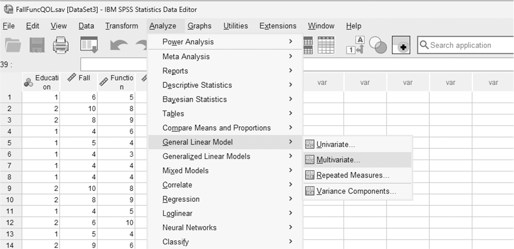
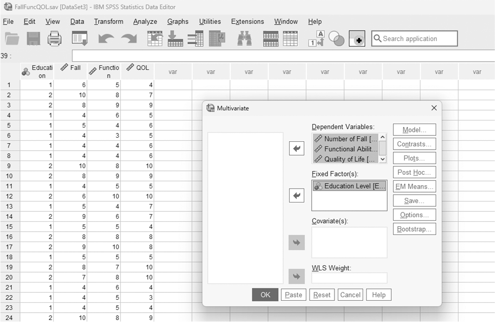
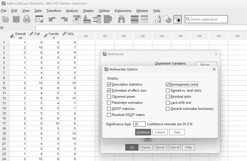
To conduct MANOVA in SPSS, you will open FallFuncQOL.sav and go to Analyze > General Linear Model > Multivariate, as presented in Figure 13-23. In the Multivariate dialogue box, move the independent variables into "Fixed Factor(s)" and the dependent variables into "Dependent Variables" by clicking the corresponding arrow buttons in the middle (refer to Figure 13-24). Notice that the space for dependent variables is wider than in univariate general linear models. The box has six buttons, but only commonly used buttons are discussed here. The "Contrasts" and "Post Hoc" buttons are used when further investigations are needed among more than two groups in the factor with an overall group difference from ANOVA results, as discussed earlier in this chapter. However, we do not have to use these buttons since we have only two groups. The "Options" button provides several options that may help us interpret the results of MANOVA; these are displayed in Figure 13-25. Clicking "OK" will then produce the requested output of the MANOVA analysis. An example output is presented in Table 13-7.

Selecting MANOVA under "General Linear Model" in SPSS.

A screenshot displays the SPSS interface with the Analyze menu open. The cursor points to the General Linear Model submenu, and the option Multivariate is visible in the dropdown list.

Reprint Courtesy of International Business Machines Corporation, © International Business Machines Corporation. "IBM SPSS Statistics software ("SPSS")". IBM®, the IBM logo, ibm.com, and SPSS are trademarks or registered trademarks of International Business Machines Corporation.

Defining variables in MANOVA in SPSS.

A screenshot displays the Multivariate dialog box in SPSS. Boxes for dependent variables and fixed factors are shown, with a list of available variable names on the left and arrow buttons used to assign them.

Reprint Courtesy of International Business Machines Corporation, © International Business Machines Corporation. "IBM SPSS Statistics software ("SPSS")". IBM®, the IBM logo, ibm.com, and SPSS are trademarks or registered trademarks of International Business Machines Corporation.

Useful options for MANOVA in SPSS.

A screenshot displays the SPSS options window containing checkboxes for descriptive statistics, parameter estimates, and homogeneity tests, with Continue and Cancel buttons at the bottom.

Reprint Courtesy of International Business Machines Corporation, © International Business Machines Corporation. "IBM SPSS Statistics software ("SPSS")". IBM®, the IBM logo, ibm.com, and SPSS are trademarks or registered trademarks of International Business Machines Corporation.

Table 13-7 Example Output of MANOVA in SPSS

Between-Subjects Factors

Value Label

N

Education Level

1

APRN

59

2

RN/BSN

41

Multivariate Testsa

Effect

Value

F

Hypothesis df

Error df

Sig.

Partial Eta-Squared

Intercept

Pillais Trace

.978

1454.679b

3.000

96.000

<.001

.978

Wilks Lambda

.022

1454.679b

3.000

96.000

<.001

.978

Hotellings Trace

45.459

1454.679b

3.000

96.000

<.001

.978

Roys Largest Root

45.459

1454.679b

3.000

96.000

<.001

.978

Education

Pillais Trace

.621

52.336b

3.000

96.000

<.001

.621

Wilks Lambda

.379

52.336b

3.000

96.000

<.001

.621

Hotellings Trace

1.636

52.336b

3.000

96.000

<.001

.621

Roys Largest Root

1.636

52.336b

3.000

96.000

<.001

.621

a. Design: Intercept + Education

b. Exact statistic

Levenes Test of Equality of Error Variancesa

Levene Statistic

df1

df2

Sig.

Number of Falls

Based on Mean

.138

1

98

.711

Based on Median

.262

1

98

.610

Based on Median and with adjusted df

.262

1

97.361

.610

Based on trimmed mean

.229

1

98

.633

Functional Ability

Based on Mean

.913

1

98

.342

Based on Median

.596

1

98

.442

Based on Median and with adjusted df

.596

1

97.721

.442

Based on trimmed mean

.656

1

98

.420

Quality of Life

Based on Mean

10.328

1

98

.002

Based on Median

7.902

1

98

.006

Based on Median and with adjusted df

7.902

1

87.633

.006

Based on trimmed mean

9.957

1

98

.002

Tests the null hypothesis that the error variance of the dependent variable is equal across groups.

a. Design: Intercept + Education

Tests of Between-Subjects Effects

Source

Dependent Variable

Type III Sum of Squares

df

Mean Square

F

Sig.

Partial Eta-Squared

Corrected Model

Number of Falls

200.255a

1

200.255

68.203

<.001

.410

Functional Ability

117.749b

1

117.749

49.154

<.001

.334

Quality of Life

140.701c

1

140.701

54.600

<.001

.358

Intercept

Number of Falls

4290.495

1

4290.495

1461.252

<.001

.937

Functional Ability

4251.429

1

4251.429

1774.744

<.001

.948

Quality of Life

4059.301

1

4059.301

1575.247

<.001

.941

Education

Number of Falls

200.255

1

200.255

68.203

<.001

.410

Functional Ability

117.749

1

117.749

49.154

<.001

.334

Quality of Life

140.701

1

140.701

54.600

<.001

.358

Error

Number of Falls

287.745

98

2.936

Functional Ability

234.761

98

2.396

Quality of Life

252.539

98

2.577

Total

Number of Falls

4584.000

100

Functional Ability

4487.000

100

Quality of Life

4312.000

100

Corrected Total

Number of Falls

488.000

99

Functional Ability

352.510

99

Quality of Life

393.240

99

a. R-Squared = .41O (Adjusted R-Squared = .404)

b. R-Squared = .334 (Adjusted R-Squared = .327)

c. R-Squared = .358 (Adjusted R-Squared = .351)

Descriptive Statistics

Education Level

Mean

Std. Deviation

N

Number of Falls

APN

5.22

1.692

59

RN/BSN

8.10

1.744

41

Total

6.40

2.220

100

Functional Ability

APN

5.53

1.443

59

RN/BSN

7.73

1.689

41

Total

6.43

1.887

100

Quality of Life

APN

5.27

1.298

59

RN/BSN

7.68

1.968

41

Total

6.26

1.993

100

The output indicates that the independent variable, nurses' education level, has a substantial effect on the combined dependent variables of number of falls, functional ability, and quality of life, with a small p-value of .000. Note that the output reports four different statistics for the effect of the independent variable: Pillai's trace, Wilks' lambda, Hotelling's trace, and Roy's largest root. These statistics will report the same results in most situations with relative robustness to the violation of multivariate normality, as in our output. However, there may be some cases where not all statistics agree on the significance of the independent variables. If the statistics are dissimilar, the decision can be made based on which set of dependent variables the group differences occur, but refer to previous research for further discussion (Olson, 1974, 1976; Stevens, 1980). Separate univariate ANOVAs performed as a follow-up test indicated that nurses' education level substantially affected all dependent variables. From Table 13-7, we can understand that nurses' education level substantially affected the number of falls, functional ability, and quality of life, with a small p-value of .000.

Reporting MANOVA

Reporting MANOVA results is a bit different from reporting a one-way ANOVA results because it uses different statistics. You should include one of the four multivariate statistics that are reported in the output along with the size of F-statistics, associated degrees of freedom, and the associated p-value. The computation of effect size for a MANOVA design is fairly complicated and more cumbersome than that for one-way ANOVA, but we can obtain and report estimates of effect size, partial h2, as presented in Figure 13-25. We recommend that you compute and interpret in consultation with a statistician for the other types of effect sizes.

The follow-up ANOVAs' results are reported as demonstrated previously.

The following is a sample report from our example:

There was a substantial effect of nurses' education level on the combined dependent variables, including number of falls, functional ability, and quality of life, Λ = 0.38, F (3, 96) = 52.34, p< .001, η2 = .621. Follow-up separate univariate ANOVAs revealed that nurses' education level had a substantial effect on all of the dependent variables: number of falls, F (1, 98) = 68.20, p< .001, η2 = .410, functional ability, F (1, 98) = 49.15, p< .001, η2 = .334, and quality of life, F (1, 98) = 54.60, p< .001, η2 = .358.

Note that we have reported on Wilks' lambda, but you could choose the others. You will have to ensure that you use the corresponding symbol to report (i.e., V for Pillai's trace, T for Hotelling's trace, and Θ for Roy's largest root).

Nurse investigators occasionally encounter studies and analyses that include an extension of MANOVA, multivariate analysis of covariance (MANCOVA), and factorial MANOVA. While this discussion is beyond the scope of our text, you should understand that MANCOVA is used to control for the effect of covariates on the combination of dependent variables and factorial MANOVA is used to investigate both the main and interaction effect of independent variables on a combination of dependent variables.

Summary

In this chapter, we have discussed how to carry out advanced ANOVA analyses to compare means. Occasionally, it will be important to control other variables that may influence the dependent variable, and we can accomplish this by employing ANCOVA. Other variations of ANOVA include factorial and repeated measures, which are specialized applications of one-way ANOVA that are applicable when there are multiple independent variables or the same variable is being measured over time. MANOVA allows us to analyze the effects of the grouping variable(s) on more than one dependent variable.

All these techniques share similar assumptions related to normality, independence, and homogeneity of variance. Once we have examined the effect of the independent variable(s) on the dependent variable(s), we also need to conduct follow-up statistical tests that indicate more specifically what groups are creating the effect.

Tests of differences between means are most useful in descriptive comparative and experimental designs in which differences between groups are of interest.

Critical Thinking Questions

  1. What are the differences among one-way ANOVA, factorial ANOVA, repeated measures ANOVA, ANCOVA, and multivariate ANOVA?

  2. Why is ANCOVA a more powerful design than one-way ANOVA when there is a third variable that is affecting a relationship between the independent and dependent variables?

  3. How do substantial interaction effects influence the interpretation of main effects in factorial ANOVA?

  4. What would you conclude if there is a significant interaction effect but no significant main effects in a factorial ANOVA? How would you interpret this in a nursing intervention study?

  5. In a longitudinal nursing study, how would you justify the use of repeated measures ANOVA over a series of paired t-tests?

  6. How would you determine whether the use of MANOVA is more appropriate than separate univariate ANOVAs for a nursing study with multiple outcomes?

  7. If you find a significant multivariate effect in MANOVA but not in the univariate tests, how would you explain this discrepancy?

  8. If both main effects and interaction effects are significant in a factorial ANOVA, how would you prioritize which effects to discuss in the context of a nursing intervention?

  9. What additional information does MANOVA provide compared to running multiple univariate ANOVAs, and how might this affect your interpretation of the results?

  10. If your covariate is not significantly correlated with the dependent variables in ANCOVA, how would this affect the interpretation of your findings?

Self-Quiz

  1. Suppose that you plan to compare systolic blood pressure between three age groups (50-65 years, 66-80 years, and 80 years and older), and evidence from the literature suggests that age may influence blood pressure. What statistical test will be most appropriate?

    1. One-way ANOVA

    2. Analysis of covariance

    3. Independent t-test

    4. MANOVA

  2. Suppose that you find that there is an interaction effect of gender and ethnicity on risk for falls in a nursing home. What statistic will help you determine which variable is contributes the greatest variance?

    1. Simple effect analysis

    2. Bonferroni test

    3. Levine's test for homogeneity

  3. Suppose that you find that there is a substantial effect of the independent variable on the set of four dependent variables. Which tests can you conduct to follow up the substantial results?

    1. A series of ANOVAs

    2. Roy-Bargman stepdown analysis

    3. Discriminant analysis

    4. All of these are correct.

  4. True or False: A factorial ANOVA allows the examination of both main effects and interaction effects simultaneously.

  5. True or False: A statistically significant MANOVA result implies that each individual dependent variable is significantly different across groups.

  6. In a factorial ANOVA, an interaction effect indicates that:

    1. the effect of one independent variable depends on the level of another independent variable.

    2. all independent variables have equal effects.

    3. main effects are always significant.

    4. no post hoc tests are required.

  7. True or False: Repeated measures ANOVA is appropriate for analyzing data where the same subjects are measured multiple times.

  8. What assumption is specific to repeated measures ANOVA that must be tested?

    1. Homogeneity of variances

    2. Sphericity

    3. Multicollinearity

    4. Independence of observations

  9. If the sphericity assumption is violated in a repeated measures ANOVA, what adjustment should be made?

    1. Use a Bonferroni correction.

    2. Apply the Greenhouse-Geisser correction.

    3. Conduct a paired t-test.

    4. Ignore the violation.

  10. True or False: If the dependent variables are highly correlated, running separate ANOVAs is preferable to using MANOVA.

Reference

OlsonC. L. (1974). Comparative robustness of six tests in multivariate analysis of variance. Journal of the American Statistical Association, 69, 894-908.OlsonC. L. (1976). On choosing a test statistic in multivariate analysis of variance. Psychological Bulletin, 83, 579-586.StevensJ. P. (1980). Power of the multivariate analysis of variance tests. Psychological Bulletin, 88, 728-737.WatkinsS., AstrothK. S., KimM., & DyckM. J. (2023). Effects of Medicare wellness visits on health promotion outcomes. Journal of the American Association of Nurse Practitioners, 35(2), 104-111. https://doi.org/10.1097/JXX.0000000000000795