section name header

Learning Objectives

This chapter explains how to conduct and interpret analyses of associations between two categorical variables. By the end of this chapter, you will be able to:

Key Concepts and Terms

Introduction

Nurses are often interested in relationships between variables. Such investigations are important steps in the development of interventions that are used to improve patient outcomes. When variables are measured at the interval or ratio level (also called continuous variables), we use Pearson's r to examine the relationship between variables. However, some variables of interest are categorical in nature (i.e., nominal or ordinal), such as patient outcomes (improved/not improved), diagnoses (presence/absence of a condition), or demographic categories (race, gender identity).

Case Studies

Badger, T. A., Segrin, C., Crane, T. E., Chalasani, P., Arslan, W., Hadeed, M., & Sikorskii, A. (2023). Social determinants of health and symptom burden during cancer treatment. Nursing Research, 72(2), 103-113. https://doi.org/10.1097/NNR.0000000000000636

Badger et al. (2023) explored the impact of social and demographic factors on symptoms of patients with cancer undergoing treatment. Sociodemographic characteristics selected for this study were age, sex, number of comorbid conditions, race, ethnicity, marital status, employment, income, health insurance, urban or rural residence, cancer site, cancer recurrence, and metastasis. Symptoms were identified using instruments to evaluate depression, anxiety, common distressing symptoms, social isolation, and a Hispanic patient acculturation score.

The researchers conducted a secondary analysis of data from 400 cancer survivors who participated in a randomized controlled trial. Race and ethnicity data were condensed to three groups (Hispanic [n = 168], non-Hispanic White [n = 191], and non-Hispanic others [n = 41]) for comparison. Chi-square tests (χ2) were used to evaluate categorical variables (e.g., number of comorbid conditions, social isolation, level of education, availability of health insurance). Continuous variables (e.g., age) were examined using analyses of variance.

Results indicated that of the three groups, non-Hispanic White patients were older with more education (p< .01) and income (p< .01), and had more comorbid conditions (p = .01) and metastatic cancers (p = .02). Hispanic patients experienced the least availability of health insurance (p = .01). Non-Hispanic others had lower social isolation levels (p< .01). There was a statistically significant relationship between age, quantity of comorbid conditions, social isolation with depression, frequency and severity of symptoms. Other associations include age and social isolation with anxiety. Symptom severity was lowest in non-Hispanic White patients.

Overall, Badger et al. (2023) found important associations of age, income, social isolation, and residence with distressing symptom quantity and severity, depression, and anxiety. These findings may assist clinicians in identifying patients with cancer who could benefit from additional support to improve their treatment experiences and outcomes.

For example, we might be interested in variables such as blood type (A, B, O, or AB), response level to treatment (recovery, disability, or death), or ethnicity. These data are measured at the nominal or ordinal level and do not lend themselves to arithmetic analyses. These types of data are often called categorical data. A categorical variable may be examined through a frequency analysis (e.g., counting the number of times the patient recovers) as we saw in Chapter 6. Still, a frequency analysis does not help us answer a more sophisticated question, such as understanding the relationship between two or more categorical variables. Crosstab analysis is a simple extension of frequency analysis that allows us to examine the association between two or more categorical variables in terms of joint frequencies. As both variables are categorical, descriptive mean and standard deviation statistics do not make sense. Instead, we analyze the frequency and/or the percentage/proportion to answer questions about associations between variables.

Investigators may examine the associations between categorical variables to understand health outcomes and diseases in relation to socioeconomic factors, race and ethnicity, geographical location, and so on. An investigator might ask a question such as, "Is there a relationship between where a patient resides (urban or rural) and their health status (excellent, good, fair, or poor)?" In this case, a variable, place of residence, is measured at the nominal level and has two possible choices; the other variable is ordinal and has four possible choices. Similarly, the nurse investigator might ask a quality improvement question such as, "What is the relationship between the presence or absence of a patient navigator (a nurse who helps patients negotiate complex health problems and treatment) and patient satisfaction (high, moderate, or low)?"

Interpreting the results of these types of studies must be made with an understanding of each approach's strengths and limitations and the statistical analysis's underlying assumptions. As a nurse investigator, you must recognize what variables are being studied, what hypotheses are proposed, and the level of measurement for each variable to choose the most appropriate statistical test for the analysis.

Chi-Square (2) Test

The chi-square test is the simplest method to analyze variables that are measured at the categorical level. The chi-square test is a type of nonparametric test that does not make a distributional assumption, making it suitable for a wide range of healthcare data. In the analysis, both Excel and IBM SPSS Statistics software (SPSS) create a crosstab between the two variables and then analyze the frequencies for a possible association. The following are example questions that can be addressed with a chi-square test:

A contingency table presents the frequency distribution of the two categorical variables, and the chi-square test can be used to test the relationship between variables for any contingency table that is 2 × 2 (i.e., both variables are dichotomous at either the nominal or ordinal level of measurement) or larger. An example of a 2 × 2 table is presented in Table 15-1. Note that in this example, there are two variables, age and antihistamine use, and each has two choices: for age, older than 30 years or younger than 30 years, and for antihistamine use, use or do not use. The 2 × 2 refers to the number of categories of variables being analyzed simultaneously (i.e., both variables are dichotomous). A 3 × 3 table might be an analysis of health status (poor, good, and excellent) by income (low, middle, and high).

Table 15-1 Example Data for Chi-Square Test

Do Not Use Antihistamines

Use Antihistamines

Total

Younger than 30

105

32

137

Older than 30

72

9

81

Total

177

41

218

Assumptions

As the chi-square test is a type of nonparametric test, it does not make distributional assumptions. However, the following assumptions apply:

  • All observations are independent.

  • Expected count or cases in each cell should be greater than 1.

  • Expected count or cases in no more than 20% of cells should be less than 5.

Doing and Interpreting Chi-Square Tests

First, we need to set up hypotheses to test the association between two categorical variables. They can be written as follows:

H0: There is no association between the two categorical variables.

Ha: There is an association between the two categorical variables.

The test statistic is calculated by the following formula:

Formula reads: Chi squared equals summation of open bracket open parenthesis Observed frequency minus Expected frequency close parenthesis squared over Expected frequency close bracket.

where the expected frequency is found by dividing the product of the raw total frequency and column total frequency with the grand total frequency. The statistic can be conceptualized as the difference between the observed and expected frequencies in each contingency table cell. For example, let us suppose an investigator is interested in examining whether one age group is more prone to use antihistamines than another. Refer to Table 15-2 for an example data set.

Table 15-2 Example Data for Chi-Square Test with Expected Frequency

Do Not Use Antihistamines

Use Antihistamines

Total

Younger than 30

105 (111.23)

32 (25.77)

137

Older than 30

72 (65.77)

9 (15.23)

81

Total

177

41

218

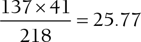
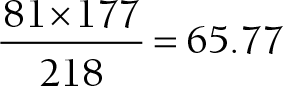
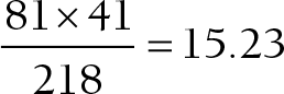
The numbers inside the contingency table represent the observed frequency (with expected frequency in parentheses). For example, there are 105 people who are younger than 30 years and do not use antihistamines, 32 who are younger than 30 years and use antihistamines, 72 who are older than 30 years and do not use antihistamines, and 9 who are older than 30 years and use antihistamines. We need to calculate the expected frequency to be able to compute the chi-square statistic as displayed in the previous equation, and it is the ratio of the raw total frequency multiplied by the column total frequency over the grand total frequency. For example, the expected frequency of all four cells will be the following:

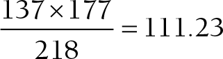
Calculation reads: 137 times 177 over 218 equals 111.23.

Calculation reads: 137 times 41 over 218 equals 25.77.

Calculation reads: 81 times 177 over 218 equals 65.77.

Calculation reads: 81 times 41 over 218 equals 15.23.

Then, the chi-square statistic is
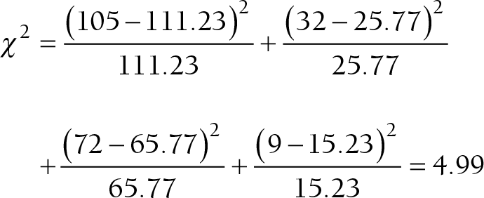
Calculation reads: Chi squared equals open bracket open parenthesis 105 minus 111.23 close parenthesis squared over 111.23 close bracket plus open bracket open parenthesis 32 minus 25.77 close parenthesis squared over 25.77 close bracket plus open bracket open parenthesis 72 minus 65.77 close parenthesis squared over 65.77 close bracket plus open bracket open parenthesis 9 minus 15.23 close parenthesis squared over 15.23 close bracket equals 4.99.

Once the statistic is computed, we evaluate the associated p-value with the statistic, and we decide to reject or not reject the null hypothesis. We reject the null hypothesis when the p-value associated with the computed statistic is small, and we do not reject it when the p-value associated with the computed statistic is large.

For our example, the associated p-value with the statistic of 4.99 is .025. Because this indicates that we would expect to observe an outcome as extreme as our statistic in only about 2 or 3 samples out of 1,000, we decide to reject the null hypothesis and to conclude that age (being older or younger than 30 years) is associated with antihistamine use.

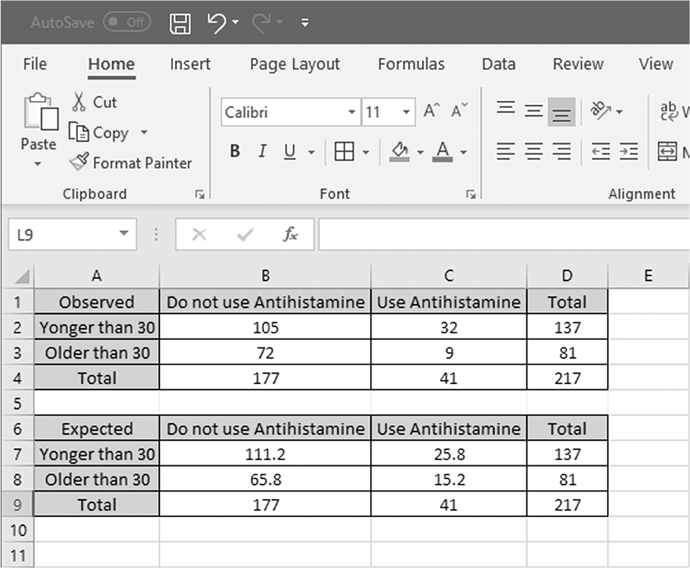
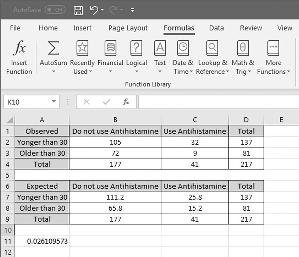
To conduct a chi-square test in Excel, you will open Antihistamin.xlsx and note that the data contain the observed frequency and the expected frequency in separate contingency tables (Figure 15-1). There are two ways to conduct a chi-square test in Excel. The first step is to go to Formulas > Insert Functions and find the chisq.test function in the "Insert Function" dialogue box (Figure 15-2). Click "OK," and then you will provide B2:C3 as Actual_Range and B7:C8 as Expected_Range (Figure 15-3) in the "Function Arguments" dialogue box. Clicking "OK" will then produce the p-value of the chi-square test for our data set (Figure 15-4). The second is to type in chisq directly.test function, and the formula for this is "=chisq.test(B2:C3,B7:C8)" (Figure 15-5). Pressing "Enter" will then produce the output of chi-square test (Figure 15-4).

Formatting the data for analysis in Excel.
An Excel screenshot shows two tables, Observed and Expected.

The first table shows four columns: Observed, Do not use Antihistamine, Use Antihistamine, and Total. The row entries are as follows. Row 1: Younger than 30, 105, 32, 137. Row 2: Older than 30, 72, 9, 81. Row 3: Total, 177, 41, 217. The second table shows four columns: Expected, Do not use Antihistamine, Use Antihistamine, and Total. The row entries are as follows. Row 1: Younger than 30, 111.2, 25.8, 137. Row 2: Older than 30, 65.8, 15.2, 81. Row 3: Total, 177, 41, 217.

Courtesy of Microsoft Excel © Microsoft 2020.

Finding chi-square function in Excel.
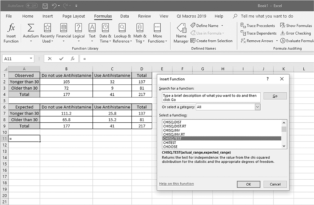
An Excel screenshot shows two tables, with numerical data. A dialog box, with heading, Insert function, shows a list of functions, of which chi-square is selected.

Courtesy of Microsoft Excel © Microsoft 2020.

Defining data ranges for "chisq.test" function in Excel.
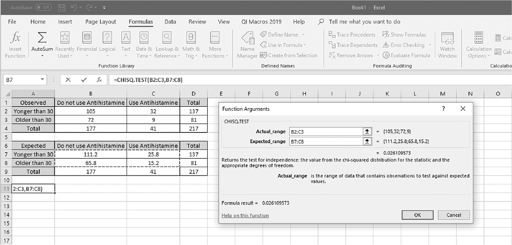
An Excel screenshot shows two tables, with numerical data. A dialog box, with heading, Function Arguments, shows values entered in the Actual_Range and Expected_Range fields.

Courtesy of Microsoft Excel © Microsoft 2020.

Example output for "chisq.test" in Excel.
An Excel screenshot shows two tables, Observed and Expected.

The first table shows four columns: Observed, Do not use Antihistamine, Use Antihistamine, and Total. The row entries are as follows. Row 1: Younger than 30, 105, 32, 137. Row 2: Older than 30, 72, 9, 81. Row 3: Total, 177, 41, 217. The second table shows four columns: Expected, Do not use Antihistamine, Use Antihistamine, and Total. The row entries are as follows. Row 1: Younger than 30, 111.2, 25.8, 137. Row 2: Older than 30, 65.8, 15.2, 81. Row 3: Total, 177, 41, 217. The value, 0.026109573, is displayed below the tables.

Courtesy of Microsoft Excel © Microsoft 2020.

Typing in "chisq.test" function with data ranges in Excel.
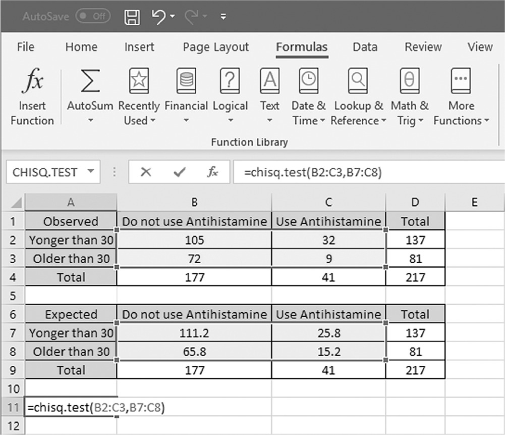
An Excel screenshot shows two tables, Observed and Expected.

The first table shows four columns: Observed, Do not use Antihistamine, Use Antihistamine, and Total. The row entries are as follows. Row 1: Younger than 30, 105, 32, 137. Row 2: Older than 30, 72, 9, 81. Row 3: Total, 177, 41, 217. The second table shows four columns: Expected, Do not use Antihistamine, Use Antihistamine, and Total. The row entries are as follows. Row 1: Younger than 30, 111.2, 25.8, 137. Row 2: Older than 30, 65.8, 15.2, 81. Row 3: Total, 177, 41, 217. The formula, chi-squared test of B 2 to C 3, B 7 to C 8, is displayed below the tables.

Courtesy of Microsoft Excel © Microsoft 2020.

To conduct a chi-square test in SPSS, you will open Antihistamine.sav and go to Analyze > Descriptive Statistics > Crosstabs, as displayed in Figure 15-6. In the Crosstabs dialogue box, insert one of the variables into the "Row(s)" box and the other into the "Column(s)" box (Figure 15-7). Click on the "Statistics" button, which allows you to conduct various statistical tests, but notice that none are checked by default in the Crosstabs Statistics dialogue box. Click on "Chi-square," as displayed in Figure 15-8. This will perform the actual test and produce the results of significance testing. Clicking "Continue" and then "OK" will produce the output. The example output is presented in Table 15-3.

Selecting a chi-square test in SPSS.
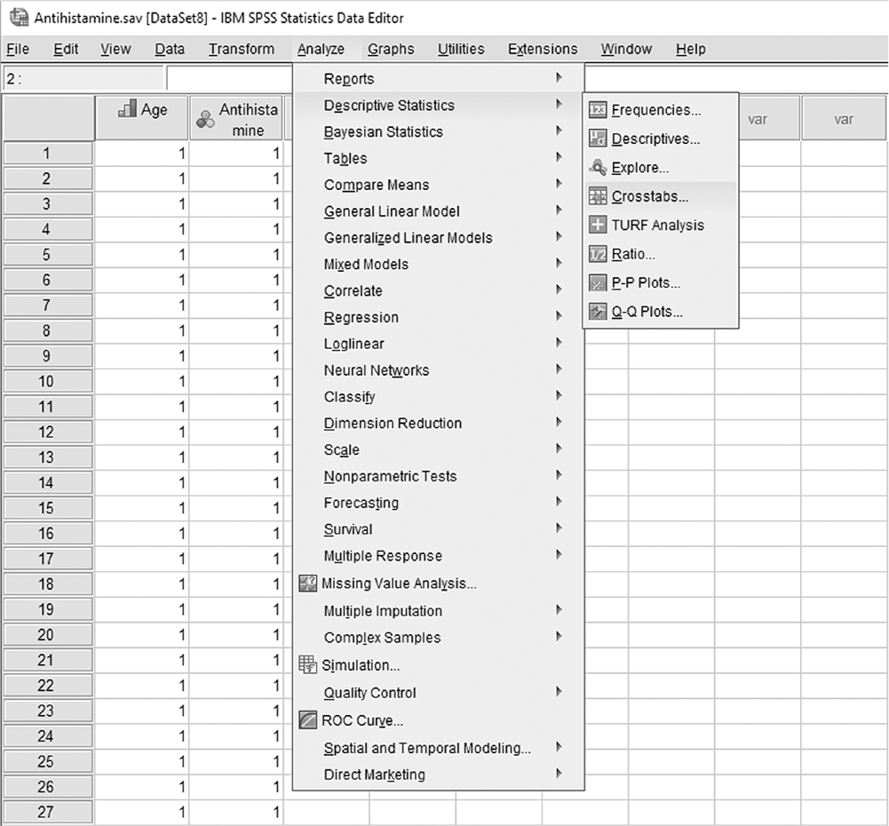
A screenshot in S P S S shows selection of the Analyze menu, with Descriptive Statistics command chosen, from which Crosstabs option is selected. Data in the worksheet shows columns of numerical data.

Reprint Courtesy of International Business Machines Corporation, © International Business Machines Corporation. "IBM SPSS Statistics software ("SPSS")". IBM®, the IBM logo, ibm.com, and SPSS are trademarks or registered trademarks of International Business Machines Corporation.

Defining variables in chi-square tests in SPSS.
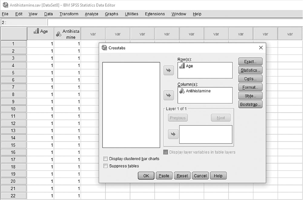
A screenshot in S P S S Editor defines variables in Chi-square tests. The data in the worksheet shows columns of numerical data.

The dialog box, with heading, Crosstabs, shows an empty box on the left. Three arrow buttons follow this. There are three boxes to the right of the arrow buttons, which are as follows from top to bottom: Rows, Columns, and Layer 1 of 1. Below are three options: Display layer variables in table layers, Display clustered bar charts, and Suppress tables, of which Display layer variables in table layers is greyed out. The buttons, Exact, Statistics, Cells, Format, and Bootstrap, are present in the right side of the dialog box; the buttons, Ok, Paste, Reset, Cancel, and Help are present at the bottom of the dialog box.

Reprint Courtesy of International Business Machines Corporation, © International Business Machines Corporation. "IBM SPSS Statistics software ("SPSS")". IBM®, the IBM logo, ibm.com, and SPSS are trademarks or registered trademarks of International Business Machines Corporation.

Checking options in chi-square tests in SPSS.
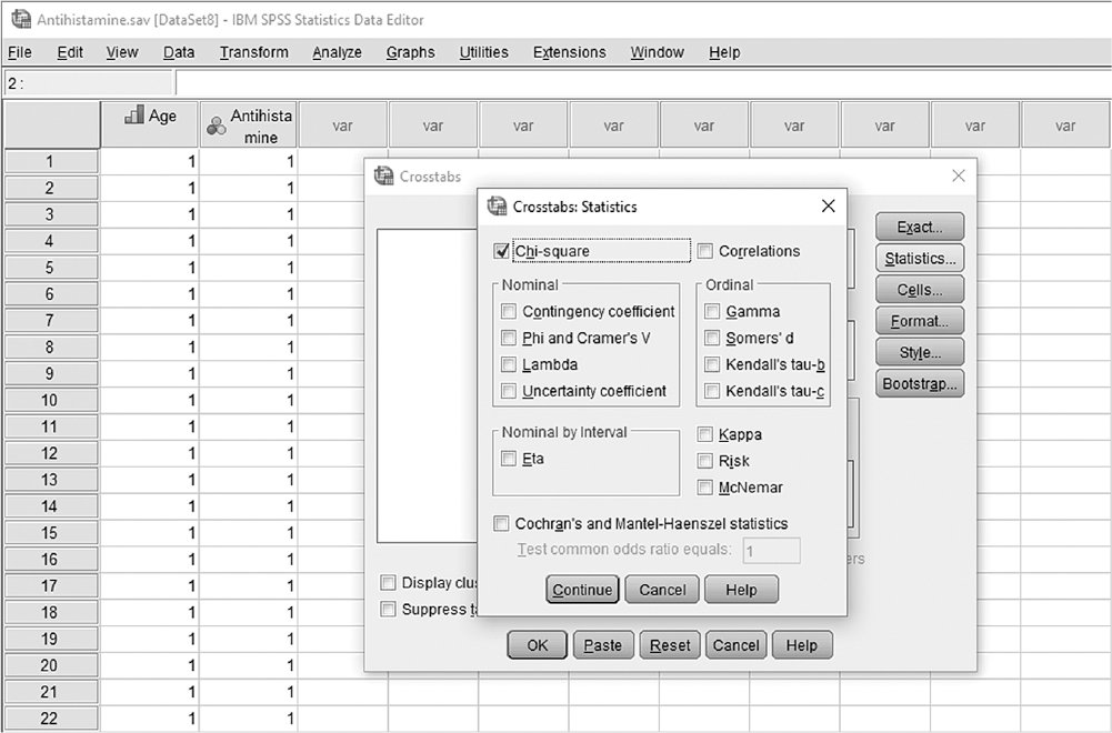
A screenshot in S P S S shows two columns of numerical data. A dialog box, with heading Crosstabs Statistics, shows several options listed; the option chi-square is checked.

Reprint Courtesy of International Business Machines Corporation, © International Business Machines Corporation. "IBM SPSS Statistics software ("SPSS")". IBM®, the IBM logo, ibm.com, and SPSS are trademarks or registered trademarks of International Business Machines Corporation.

Table 15-3 Example Output of Chi-Square Tests in SPSS

Case Processing Summary

Cases

Valid

Missing

Total

N

Percent

N

Percent

N

Percent

Age* antihistamine

218

100.0

0

.0

218

100.0

Age* Antihistamine Crosstabulation Count

Antihistamine

Do Not Use Antihistamine

Use Antihistamine

Total

Age

Younger than 30

105

32

137

Older than 30

72

9

81

Total

177

41

218

Chi-Square Tests

Value

df

Asymp. Sig. (2-Sided)

Exact Sig. (2-Sided)

Exact Sig. (1-Sided)

Pearson chi-square

5.000a

1

.025

Continuity correctionb

4.230

1

.040

Likelihood ratio

5.323

1

.021

Fishers exact test

.031

.018

Linear-by-linear association

4.977

1

.026

N of valid cases

21.8

a0 cells (.0%) have expected count less than 5. The minimum expected count is 15.23.

bComputed only for a 2 × 2 table.

Reporting Chi-Square Tests

When reporting chi-square test results, you should report the size of corresponding chi-square statistics with its associated degrees of freedom and p-value. The following is a sample report from our example:

  • There was an association between the age group and whether or not they use antihistamines, χ2 (1) = 5.00, p = .025.

In this case, the degrees of freedom are equal to (r 1) × (c 1), where r is the number of rows and c is the number of columns in the contingency table. Therefore, we get (2 1) × (2 1) = 1.

Fisher's Exact Test

One of the assumptions of a chi-square test was that the expected count in all cells should be greater than 1 and no more than 20% of cells should have a count of less than 5. The chi-square test becomes unstable (a less reliable and less valid analytic tool) when this assumption is violated (i.e., expected count in any cell is small). Fisher (1922), the famous statistician, developed Fisher's exact test to resolve this problem. Note that Fisher's exact test should only be used with 2 × 2 contingency tables when the sample size is small enough that the assumption can be violated. As we have seen in Table 15-3, the output of the chi-square test reports additional statistics, including Fisher's exact test.

Let us consider the following output where we have slightly modified the data so that some cells have an expected frequency of less than 5. That output is presented in Table 15-4. Notice that the cells for people younger than 30 who do not use antihistamines and those younger than 30 who use antihistamines have expected frequencies of less than 5, which violates the assumption. Therefore, the result of Fisher's exact test should be reported instead of that of the chi-square test. In our example, both p-values are small enough to rule out chance, so the results indicate the association between the age group and whether they use antihistamines.

Table 15-4 Example Output When Some Cells Have an Expected Frequency of Less Than 5

Age* Antihistamine Crosstabulation Count

Antihistamine

Do Not Use Antihistamine

Use Antihistamine

Total

Age

Younger than 30

1 (3.81)

7 (4.19)

8

Older than 30

9 (6.19)

4 (6.81)

13

Total

10

11

21

Chi-Square Tests

Value

df

Asymp. Sig. (2-Sided)

Exact Sig. (2-Sided)

Exact Sig. (1-Sided)

Pearson chi-square

6.390a

1

.011

Continuity correctionb

4.318

1

.038

Likelihood ratio

6.988

1

.008

Fishers exact test

.024

.017

Linear-by-linear association

6.086

1

.014

Number of valid cases

21

aExpected count is shown in parentheses, and 2 cells (50.0%) have expected count less than 5. The minimum expected count is 3.81.

bComputed only for a 2 × 2 table.

Phi and Cramer's V

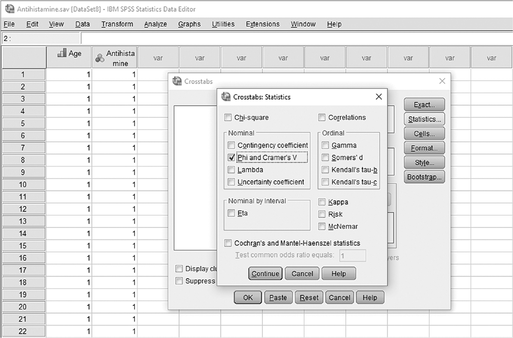
When "Chi-square" is checked in the Crosstabs Statistics dialogue box, it calculates the statistic with its associated p-value. It indicates whether the two categorical variables are related. However, the small p-value associated with the chi-square statistic only indicates that the variables are related; it does not reveal anything about the strength of the relationship. In the Crosstabs Statistics box, there are two statistics that we can calculate and report when the strength of association is of interest; they are Phi and Cramer's V. Click on the "Statistics" button and check "Phi and Cramer's V," as displayed in Figure 15-9, to calculate measures for the strength of association between the two variables. Clicking "Continue" and then "OK" will then produce the output. The example output is presented in Table 15-5; note that this output is added to Table 15-3.

Table 15-5 Example Output of Phi and Cramer's V in SPSS

Symmetric Measures

Value

Approx. Sig.

Nominal by nominal

Phi

-.151

.025

Cramer's V

.151

.025

Number of valid cases

218

Choosing Phi and Cramer's V in chi-square test in SPSS.

A screenshot in S P S S shows two columns of numerical data. A dialog box, with heading Crosstabs Statistics, shows several options listed; the option Phi and Cramer’s V is checked.

Reprint Courtesy of International Business Machines Corporation, © International Business Machines Corporation. "IBM SPSS Statistics software ("SPSS")". IBM®, the IBM logo, ibm.com, and SPSS are trademarks or registered trademarks of International Business Machines Corporation.

Phi is used when both variables are dichotomous (when there are only two outcomes such as "yes" or "no," "present" or "not present"), but Cramer's V should be used when one of the variables is measured for more than two categories. Phi (φ) ranges between 1 and 1, and Cramer's V ranges between 0 and 1; the general rule for correlation coefficients can be used to interpret them (as discussed in Chapter 10). As the coefficient approaches 0, the association between the two categorical variables is weak but stronger as it approaches 1. Negative and positive signs will indicate whether the association is a positive or negative relationship. Note that these statistical tests can also be used to measure effect size. The reporting of these statistics can be added after the associated p-value with chi-square test statistics. Here is a sample report:

Relative Risk and Odds Ratio

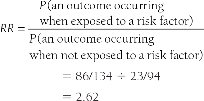
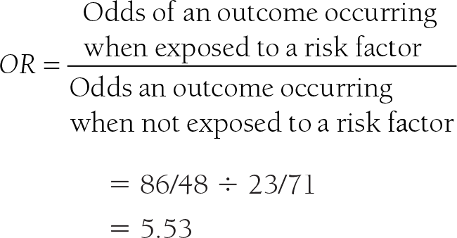
When categorical data are collected in 2 × 2 contingency tables, we can use other measures of effect size. Relative risk (RR) and odds ratio (OR) are two measures commonly used in epidemiology and clinical research to quantify the association between an exposure (e.g., a risk factor or an intervention) and an outcome (e.g., disease occurrence or recovery). Both measures help health professionals understand how likely an outcome is in one group compared to another, but they are used in different study designs. The RR is defined as the measure of the risk of an outcome (e.g., disease or death) occurring when exposed to a risk factor, and OR is defined as the ratio of an outcome (e.g., disease or death) occurring when exposed to a risk factor. For example, RR is the probability that a patient who smokes will develop lung cancer relative to that of a patient who does not smoke, and OR is the odds of a patient who smokes developing lung cancer divided by the odds of a nonsmoking patient developing lung cancer. Note that both measures can be calculated and interpreted only for 2 × 2 contingency tables.

Let us take the following example, where an association between smoking and lung cancer is examined; the data are presented in Table 15-6.

Table 15-6 The Data for Smoking and Lung Cancer

Lung Cancer

No Lung Cancer

Total

Smokers

86

48

134

Nonsmokers

23

71

94

Total

109

119

228

Then, the RR is calculated as follows:

Calculation reads: R R equals P of open parenthesis an outcome occurring when exposed to a risk factor close parenthesis over P of open parenthesis an outcome occurring when not exposed to a risk factor close parenthesis equals 86 over 134 divided by 23 over 94 equals 2.62.

and OR is calculated as follows:

Odds of an outcome occurring when exposed to a risk factor

Calculation reads: O R equals Odds of an outcome occurring when exposed to a risk factor over Odds an outcome occurring when not exposed to a risk factor equals 86 over 48 divided by 23 over 71 equals 5.53.

Interpreting both RR and OR can be done in the same manner. If either the RR or OR is equal to 1, it implies that the risk or odds of the two groups are the same in terms of an outcome occurring. If that were the case in our example, it would mean that it does not matter whether you smoke in getting lung cancer. If either the RR or OR is greater than 1, it implies that there is a positive association between the outcome occurring and exposure to a risk factor; therefore, an exposure to a risk factor will increase the occurrence of an outcome. For our example, you will be 2.62 (or 5.53 for OR) times more likely to get lung cancer if you smoke. If either RR or OR is less than 1, it implies that there is a negative association between the outcome occurring and an exposure to a risk factor. Note that a corresponding confidence interval (CI) should also be reported when both RR and the OR are reported. A report for the data in Table 15-6 is presented in the following example:

  • There was a substantial association between smoking and getting lung cancer, χ2 (1) = 34.92, p = .000. The OR was also computed for this data and indicates that the odds of getting lung cancer were 5.53 times (95% CI: 3.07, 9.96) higher for a smoking person than a nonsmoking person.

From the previous example, we saw that RR and the OR could produce different results. So, which one should we use? Both measures examine an association between exposure to a risk factor and the occurrence of an outcome, but they are not the same measures. The RR measures whether an exposure to a risk factor makes a difference in the occurrence of the outcome. In contrast, the OR measures whether there is a difference in an exposure to a risk factor in those with and without the occurrence of an outcome.

Often, the RR is an easier and more interpretable measure of an association. Still, the OR has been more widely used in statistics, particularly with logistic regression in clinical studies. The OR is commonly used for case-control studies, in which no-condition and condition groups are compared in an attempt to identify factors that may contribute to an outcome, whereas RR is commonly used in cohort studies (i.e., longitudinal analysis of risk factors) or randomized controlled trials.

Summary

The chi-square test is the preferred method to investigate an association between two categorical variables. Assumptions include independence of observations and adequate sample size for each cell. Because it has no distributional assumption, it is a nonparametric test.

In cases where any cell contains a frequency of less than 5 in 2 × 2 contingency tables, Fisher's exact test can be used and reported instead of a chi-square test because the chi-square test becomes unstable with a small sample size.

The small p-value associated with the chi-square statistic only indicates that the variables are related, so we may need a different measure of the strength of association. Phi and Cramer's V are such measures. Phi is reported for 2 × 2 contingency tables, whereas Cramer's V is reported for larger contingency tables.

RRs and ORs can also be computed and reported as effect sizes. RR is defined as the measure of the risk of an outcome (e.g., disease or death) occurring when exposed to a risk factor, and OR is defined as the ratio of an outcome (e.g., disease or death) occurring when exposed to a risk factor. Both should be reported with their associated CI.

Critical Thinking Questions

  1. Explain why the chi-square test is part of the family of nonparametric tests.

  2. An investigator found that there is an association between gender identity and pain level (low versus high) with a small p-value, and the associated Phi measure was 30. How would the researcher interpret this measure? Explain.

  3. Briefly describe a potential study in your field where you might use a chi-square test.

    1. Provide a one- or two-sentence description of the study (e.g., nature of the subjects/participants, purpose).

    2. State the research question that a chi-square test would answer.

    3. Describe the variables to be used for the chi-square test.

    4. Indicate what a low p-value associated with the chi-square test statistic in this study would state.

  4. If a new intervention for pressure ulcer prevention yields an RR = 0.5, what does that mean for patients receiving the intervention? How might this be communicated to clinicians?

  5. How would you decide between using a chi-square test of independence versus a logistic regression model for binary outcomes in a clinical study?

  6. Describe a hypothetical nursing scenario using Fisher's exact test rather than the chi-square test.

  7. In a nursing study, a statistically significant chi square was found for "smoking status" versus "postoperative complications," but Phi = 0.08. What might you conclude?

  8. If the author of a journal article reports a statistically significant chi-square value but does not provide any measure of association (like Phi or Cramer's V) or effect size, what additional questions might you ask or what additional information would you seek?

  9. In a case-control study about a rare infection, an odds ratio (OR) = 3 is found for patients exposed to a certain risk factor. How would you explain this finding to a colleague who is not statistically trained?

  10. Why might a researcher choose the chi-square test of independence instead of a t-test when comparing two groups?

Self-Quiz

  1. True or False: A chi-square test result with a small p-value will indicate that the two variables are associated and how strong a relationship is.

  2. Which of the following statistics should be reported when any cell has an expected frequency of less than 5 in a 2 × 2 contingency table?

    1. Chi-square

    2. Likelihood ratio

    3. Fisher's exact test

    4. Linear-by-linear association

  3. True or False: Cramer's V is a more appropriate measure for the strength of association than Phi when the size of a contingency table is 2 × 2.

  4. True or False: RR is used with a cohort study, whereas OR is used for a case-control study.

  5. Phi (ϕ) is typically used to measure effect size for:

    1. any size contingency table.

    2. only 2 × 3 contingency tables.

    3. specifically 2 × 2 contingency tables.

    4. ordinal data analysis.

  6. Odds ratio (OR) is best described as:

    1. the probability of an event occurring in a population.

    2. the ratio of probabilities of an event in two groups.

    3. the ratio of odds of an event in two groups.

    4. a measure exclusively used in randomized controlled trials.

  7. True or False: A Cramer's V of 0.65 indicates an extremely weak relationship.

  8. True or False: Both RR and OR compare the frequency of an outcome in exposed versus nonexposed groups, but RR directly compares risks while OR compares odds.

  9. In a case control study of patients with a rare infection (cases) and without it (controls), researchers want to see if prior exposure to a specific contaminated source is associated with the infection. Which measure of association is most appropriate?

    1. Relative risk

    2. Odd ratio

    3. Phi coefficient

    4. Cramer's V

  10. True or False: A p-value from a chi-square test of independence alone indicates whether the association is statistically significant but does not inform you of the magnitude of that association.

Reference

BadgerT. A., SegrinC., CraneT. E., ChalasaniP., ArslanW., HadeedM., & SikorskiiA. (2023). Social determinants of health and symptom burden during cancer treatment. Nursing Research , 72(2), 103-113. https://doi.org/10.1097/NNR.0000000000000636FisherR. A. (1922). On the interpretation of χ2 from contingency tables, and the calculation of P. Journal of the Royal Statistical Society, 85(1), 87-94. https://doi.og/10.2307/2340521