section name header

Learning Objectives

This chapter introduces the interpretation and application of descriptive statistics within the context of a normal distribution. By the end of this chapter, you will be able to:

Key Concepts and Terms

Introduction

We have learned how nurses in practice, leadership roles, and research can present data and statistical analyses in graphs, charts, and tables. Because the data are presented more concisely, these visual displays are handy. However, we lose the details in these displays, especially around the distribution of data that are measured at the interval and ratio level (continuous variables). Combined with the visual representation of data, we also need an approach that allows us to explore and understand the details. Descriptive statistics are used to communicate important information about the characteristics of the participants and phenomena in a study. These analyses help us answer questions such as, "What is the average length of stay in a nursing home?" "What is the range of comorbid diagnoses among patients admitted to the medical intensive care unit?" or "What is the most frequently reported reason for patients coming to urgent care?"

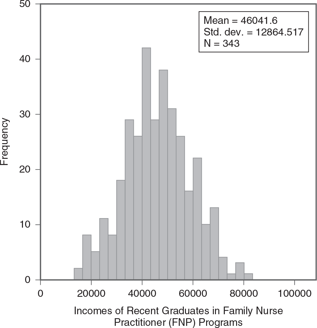
When the data are measured at the interval or ratio level, it is important to present the distribution of data in terms of central tendency (i.e., the average case) and variability (i.e., the range and spread of the data from the center). For example, Figure 7-1 presents a histogram of incomes of recent graduates in family nurse practitioner (FNP) programs. Questions we might ask about graduates are, "What would be the typical or average measurement value of a hypothetical person selected from this group?" and "How far are data values spread from the average?" These are difficult questions to answer with visual displays such as graphs, charts, and tables. We need numerical measures of central tendency and variability so that we can understand the distribution of the data on an objective basis. Descriptive statistics are numeric measurements of central tendency and variability, and they help us explain the data more accurately and in greater detail than visual displays alone.

Histogram of incomes of recent graduates in FNP programs.

A histogram shows the incomes of recent graduates in family nurse practitioner programs.

Reprint Courtesy of International Business Machines Corporation, © International Business Machines Corporation. "IBM SPSS Statistics software ("SPSS")". IBM®, the IBM logo, ibm.com, and SPSS are trademarks or registered trademarks of International Business Machines Corporation.

In this chapter, you will learn how to compute and interpret measures of central tendency and variability. We will discuss the most frequently used measures of central tendency—mode, median, and mean, and of variability—range, interquartile range, variance, and standard deviation. We will also explain the use of descriptive statistics to understand normal distributions. In normal distribution, the percentages of data values are equally dispersed from the center of the distribution. In later chapters, we will discuss many statistical procedures that assume that the data have a normal distribution.

Case Studies

McCann et al. (2024) investigated pregnant women's perceptions of birth and fetal health problems associated with the use of cigarettes and e-cigarettes during pregnancy. In this cross-sectional study, a nonrandom sample of pregnant women (n = 267) who smoked cigarettes, e-cigarettes, or both in the last 30 days completed an online survey. The authors compare the demographic characteristics of the entire sample, and three groups related to their e-cigarette use (current [45.7%], ever [39.7%], never [14.6%]) using sample size (n), percentages (%), means (M), and standard deviations (SD). For example, e-cigarette current users (M = 30.1, SD = 5.3) were older than ever users (M = 28.0, SD = 5.6, p = .017).

Measures of central tendency and variance present the differences in perceptions of the three groups about harm with e-cigarette use, birth and fetal problems with cigarette use, and birth and fetal problems with e-cigarette use. Current e-cigarette users rate cigarette use absolute fetal harm as higher (M = 4.15, SD = 0.97) and e-cigarette use relative harm as lower (M = 2.86, SD = 1.37) than the other two groups (past - M = 3.91, SD = 1.04; never - M = 3.54, SD = 1.05).

In an analysis of perceived birth and fetal health outcomes, the authors present mean (M), standard deviation (SD), and measures of significance (discussed in later chapters). When participants respond to questions about the frequency of birth and fetal problems with cigarette use, current e-cigarette users rate health problems (miscarriage, sudden infant death syndrome [SIDS], low birth weight, reduced lung function, cleft palate, reduced brain function, and attention-deficit/hyperactivity disorder [ADHD]) significantly higher than the other two groups. Additionally, e-cigarette users identified the frequency of these health problems with e-cigarette use as higher than the other two groups. However, this was not significant.

This study describes the perceptions of pregnant women who have smoked in the last month about potential birth and fetal health problems with the use of cigarettes and e-cigarettes. These results may help nurses tailor their communication with pregnant women not only about the risks of cigarette use but also about e-cigarette use.

Measures of Central Tendency

We often encounter descriptions of central tendency, or averages, in reports of studies in journals. Consider two examples. Participants were, on average, 88 years old (Pillemer et al., 2024). The median number of beds was 49 (Hua et al., 2024). These authors all used a single number to describe an important aspect of data—an average. There are multiple ways of computing and presenting averages, but we will describe the three most common measures of central tendency: mode, median, and mean.

The Mode

The mode is simply the most frequently occurring number in a given data set. Let us examine the following data set of seven systolic blood pressure (SBP) measurements.

120 114 116 117 114 121 124

Notice that 114 appears twice and all other measurements appear only once. Therefore, the SBP measurement of 114 is the mode in this data set because it is the most frequently occurring value. This particular distribution of SBPs may be described as a unimodal distribution because there is only one mode. However, it is possible to have more than one mode in a data set. To explain, let us examine the following data set.

117 120 114 116 117 114 121 124

This data set has two modes, 114 and 117, because they each appear twice and the others appear only once. A data set with two modes is a bimodal distribution, and a multimodal distribution is a distribution with more than two modes.

As you probably noticed, the mode is useful primarily for variables measured at the nominal level because it is merely the most frequently occurring number in the data set. For example, if we have assigned the following numbers to the sex of participants: 1 for designated male and 2 for designated female, and out of a sample of 100, there are 75 females, the mode is 2. The mode will not be useful with continuous levels of measurement, or as the data set gets larger.

The Median

The median is the exact middle value in a distribution and divides the data set into two exact halves. Let us consider the following data set that consists of five income levels for registered nurses:

35,000 39,500 42,000 47,500 52,000

In this data set, the value of 42,000 is the median because it divides the data set into exactly two halves, with an equal number of values below and above. It was easy to find the median in this data set, but notice that this data set is ordered from the smallest to the largest data value. Consider the following data set:

47,500 39,500 32,000 52,500 42,000

It does not make sense to report 32,000 as the median because it is the smallest data value in this data set. Ordering the data from the smallest to the largest (or vice versa) is the first and the most important step in finding the median of any data set. After ordering the values, it is easy to determine that the median for this data set should be 42,000.

Notice also that the previous two data files had odd numbers of data values. Finding the median in a data set with an odd number of values is easy because you will end up with an equal number of data values above and below the median. However, it is more challenging to find the median when there are an even number of data values in the data set. Consider the following data set:

24 29 32 35 39 40

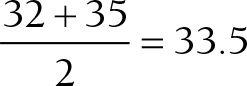
The data values represent the age in years of six individuals, and there is no number that divides this data set into two exact halves. Theoretically, such a number should be between 32 and 35, leaving three data values above and below. However, such a number does not actually exist in the data set. In this case, you must calculate the median by summing the two middle numbers, 32 and 35, and dividing the sum by 2. You are basically computing the average of those two middle values as the median, as follows:

Calculation reads: (32 plus 35) over 2 equals 33.5.

Remember that we still must order the data from the smallest to the largest value before finding a median.

The Mean

The arithmetic mean (often called the average) is the sum of all the data values in a data set divided by the number of data values and is displayed in the following equation:

Formula reads: Mean equals Sum of all data values over Number of data values.

The mean involves the mathematical operations of addition and division, and so is an appropriate measure of central tendency for interval and ratio levels of measurement. For example, we might use it to calculate an average of a patient's SBP over time to determine the effect of medication. However, it is not possible to find a meaningful interpretation for an arithmetic mean for categorical, or nominal, variables, such as political affiliation, with categories of Republican, Independent, and Democratic. Let us consider the following data set of sodium content levels, measured in milligrams per liter:

20 18 16 22 27 11

For this data set, the mean will be:

Calculation reads: Open parenthesis 20 plus 18 plus 16 plus 22 plus 27 plus 11 close parenthesis over 6 equals 19.

We have computed a mean of 19 for a group of 6 sodium content levels. How should we interpret this finding? Remember that the mean is the average score in the data set. Therefore, the mean tells us that, on average, the sodium content level in this data set is 19 mg per liter.

Choosing a Measure of Central Tendency

We have discussed three types of central tendency—the mode, the median, and the mean—and examined how they differ in terms of finding the center of a data distribution. The next legitimate question is, "When do we use which measure?"

The mode is simply the most frequently occurring data value(s) in the data set. Therefore, it is mainly useful for variables at the nominal level of measurement. Both median and mean are useful when the variable being measured can be quantified at the interval or ratio level. However, one important thing to note here is that the mean is extremely sensitive to unusual cases. To explain this further, let us consider the following data sets:

Data set #1: 108 112 116 120 124

Data set #2: 108 112 116 120 205

In both data sets, the median is 116, as it is the number that divides the data set into two exact halves. However, you will notice that the mean is not identical in both data sets.

For the first data set, the mean is equal to:

Calculation reads: open parenthesis 108 plus 112 plus 116 plus 120 plus 124 close parenthesis over 5 equals 116.

whereas the mean of the second data set is equal to

Calculation reads: open parenthesis 108 plus 112 plus 116 plus 120 plus 205 close parenthesis over 5 equals 132.2.

Notice how the mean of the second data set is influenced by the presence of an unusual case in the data set. If we were to say that the mean is equal to 132.2 for the second data set and it represents a typical case, this would not make much sense because the majority of data values are less than 120. Therefore, the mean should not be used when unusual or outlying data values are present in the data set, as the mean tends to be extremely sensitive to unusual values. Rather, the median should be reported in this case. This is why the average housing price is always reported with the median because even a single million-dollar house can distort the average housing price when most of the houses are in the range of $200,000 to $350,000. Other examples include income with a few extremely high incomes, hospital length of stays with a few patients who have significantly long stays, and any distribution that is skewed such as the distribution of wait times at a busy hospital where most patients are treated quickly but a few have extremely long waits.

Measures of Variability

Measures of central tendency allow us to know the typical value in the data set. However, we know that when we measure a variable, there will be differences among the values in the data set. For example, if we were measuring systolic blood pressure (SBP)among a group of study participants, we would expect that there would be a range of values among individuals. Furthermore, we would also expect similar variations in SBP measurements over different times in any individual participant. In other words, some level of variation among data values in any data set is expected. Our understanding of the characteristics of the data is enhanced when we also understand the nature of variability in the data set. For example, if a sample of patients has a mean SBP of 130 mm and most patients are within 10 mm of that value, then that data set will appear very different than if most patients are within 50 mm of the mean. Whenever we measure central tendency, we also need to calculate variability to achieve a thorough grasp of the data.

We also use measures of variability to provide information about how well a measure of central tendency represents the "middle/average" value in the data set. The computed measure of central tendency will be most accurate when the data values vary only a little, but the accuracy of the mean declines as the variation in data values increases. There are multiple ways of computing and presenting variability, but we describe the four that are most commonly used: range, interquartile range, variance, and standard deviation.

Range

Range is simply the difference between the largest and the smallest values in the data set. For example, suppose that a researcher measured patients' level of pain after vascular surgery on a scale of 0 to 10. This data set is:

9 3 2 6 7 8 7 5

The first step is to sort the data from the smallest to the largest values, as it will make our job of finding these two values easy. After sorting, the range of this data set is 9 2 = 7.

Range is simple to calculate. As the previous example demonstrates, the range is calculated simply by subtracting the smallest value from the highest value. However, we should be cautious about using range as a measure of variability, as it only uses the highest and lowest values in computation. In other words, the range is extremely sensitive to unusual data values. Therefore, it does not accurately capture information about how data values in the set differ if the data set contains an unusual value(s).

Consider the following data set:

3 4 2 3 3 4 2 9

This data set is still a collection of pain level measurements of patients who underwent vascular surgery, but notice that the value of 9 seems unusual in this data set. Here, the range is 9 2 = 7 after sorting. Does this make sense? Most of the values are between 2 and 4, and claiming that the variability is 7 does not really make sense in the context of this data set. To get around this problem, sometimes researchers will simply report the range as the lowest and highest values, "reports of pain intensity ranged from 3 to 9," rather than computing a range.

Interquartile Range

Interquartile range is the difference between the 75th percentile and the 25th percentile. Percentile is a measure of location and tells us how many data values fall below a certain percentage of observations. Therefore, the 25th percentile is the data value that the bottom 25% falls below, and the 75th percentile is the data value that the bottom 75% falls below. The interquartile range is less sensitive to unusual cases in the data set, as it does not use the smallest and the largest values as the standard range. For example, suppose the number of patient falls per week at a local nursing home has been measured:

1 1 2 2 2 3 3 3 4 4 5

Note that the data set has been sorted from the smallest to the largest. It is easier to find the median first and then to find the 25th and 75th percentiles because it is more difficult to directly identify the percentiles.

The median of this data set is 3, because 3 is the middle value that divides this data set into two exact halves. From the median, the 25th percentile is equal to 2, and the 75th percentile is equal to 4, as they divide the lower and upper halves of the data set into two exact halves. The interquartile range is then the difference between the 25th percentile and the 75th percentile, which is 4 2 = 2.

Let us now consider the next data set:

1 1 2 2 2 3 3 3 4 4 24

As you can identify, it is the same data set as before, except for the highest value, 24, which seems to be an unusual value. Notice that the interquartile range is still 4 2 = 2 and is not affected by the unusual data value. Therefore, the interquartile range is less sensitive to unusual or outlying values.

Variance and Standard Deviation

Although range provides a rough estimate of the variability of a data set, it does not use all of the data values in computation and is sensitive to an unusual value in the data set. Interquartile range is an improvement, but it still does not account for every data value in the set. On the other hand, the next two measures of variability, variance and standard deviation, use all the data values in the set when computing variability and may capture information about variability more precisely than the range or the interquartile range. As standard deviation is simply the square root of variance, we will explain variance first.

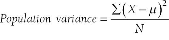
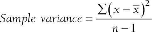
Variance is the average amount that data values differ from the mean and is computed with the following formulas:

Formula reads: Population variance equals summation of X minus mu the whole squared over N.

Formula reads: Sample variance equals summation of x minus x-bar the whole squared over open parenthesis n minus 1 close parenthesis.

In this equation, we compute the difference between each raw value and the mean (X -

), square the result, sum (Σ) those values, and then divide by the total number of values in the data set (N). Note that the denominator will be changed to n 1 when working with samples.
Degrees of Freedom

Calculations of variance and many other statistics require an estimate of the range of variability, known as degrees of freedom. Degrees of freedom refer to the number of independent values or quantities that can vary in a statistical calculation. Here is an analogy that might help you understand degrees of freedom. Envision a beverage holder from any fast-food restaurant—most of these hold four drinks. In this case, the degrees of freedom would be equal to 4 1, or 3. As each section of the holder is occupied by a drink, there is a chance of varying in what section of the holder any given drink is placed, top left or top right for example, until three of the sections are filled; at this point, there is only one section left where a drink may be placed, and no variation is possible. Each statistical test or calculation has a variation in degrees of freedom. Be mindful of these throughout the text.

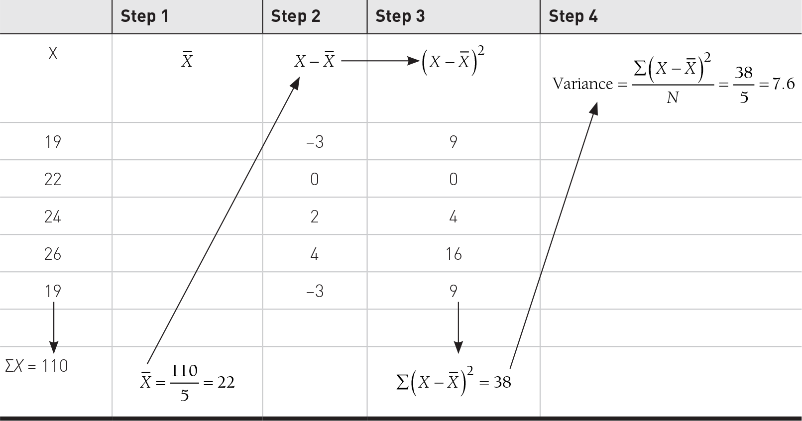
To compute variance, let us consider the following data set of toddler weights in an outpatient clinic, assuming that the data values were taken from a population:

19 22 24 26 19

The computation steps are presented in Table 7-1.

Table 7-1 How to Compute the Variance

A table is titled How to Compute the Variance.

The table consists of five columns: Blank, Step 1, Step 2, Step 3, and Step 4. The row entries are as follows. Row 1. X. X-bar. X minus X-bar. X minus X-bar the whole squared. Variance equals summation of X minus X-bar the whole squared over N equals 38 over 5 equals 7.6. Row 2. 19. Blank. Negative 3. 9. Blank. Row 3. 22. Blank. 0.0. Blank. Row 4. 24. Blank. 2. 4. Blank. Row 5. 26. Blank. 4. 16. Blank. Row 6. 19. Blank. Negative 3. 9. Blank. Row 7. Summation X equals 110. X-bar equals 110 over 5 equals 22. Blank. Summation of X minus X-bar the whole squared equals 38. Blank. Arrows point: From X-bar equals 110 over 5 equals 22 in row 7 to X minus X-bar in row 1; Summation of X minus X-bar the whole squared equals 38 in row 7 to Variance equals summation of X minus X-bar the whole squared over N equals 38 over 5 equals 7.6 in row 1; X minus X-bar in row 1 to X minus X-bar the whole squared in same row 1. An additional arrow points to Summation X equals 110 in row 7.

Computed variance for this data set is 7.6. What does this mean? Recall that the values represent toddler weights in an outpatient clinic, measured in pounds. Because the deviation of each observation from the mean has been squared, the unit for the variance is now in (pound)2. What does (pound)2 mean? If we were to say that data values differ from the mean on average by about 7.6 (pound)2, would this claim make sense? The claim does not make sense because there is no such unit as (pound)2.

Why do we then take the square of the deviation if the (unit)2 will not make sense to interpret at the end? The answer is simple: If you do not square the deviation and sum each deviation, it will always add up to zero, no matter what data set you work with. We suggest that you try this with small data sets in this text or other sources.

How can we then talk about variability if the measure of variability turns out to be equal to zero? This is why we take the square of the deviation to compute the variance first, and then take the square root of the variance to compute the standard deviation, bringing us back to the original unit of measurement.

By taking the square root of 7.6, we compute a standard deviation of 2.76. We can then say that the data values differ from the mean (22 pounds) by an average of 2.76 pounds. We can interpret this finding to mean that, on average, about two-thirds of toddlers' weights fall between 19.24 and 24.76 pounds. This makes more sense when you examine the data set compared with the variance. Note that the mean and standard deviation should always be reported together.

Choosing a Measure of Variability

We have explained you how to compute four measures of variability—range, interquartile range, variation, and standard deviation—and how they differ. The next question to ask is, "When do we use which measure?"

You should use the range only as a crude measure because it is extremely sensitive to unusual values in the data set. The interquartile range is not as sensitive to unusual data values, and the standard deviation is very sensitive to unusual values. Therefore, the interquartile range should be used with the median when the data contain unusual data values. However, the standard deviation should be used with the mean when the data are free of unusual data values.

Obtaining Measures of Central Tendency and Variability in Excel

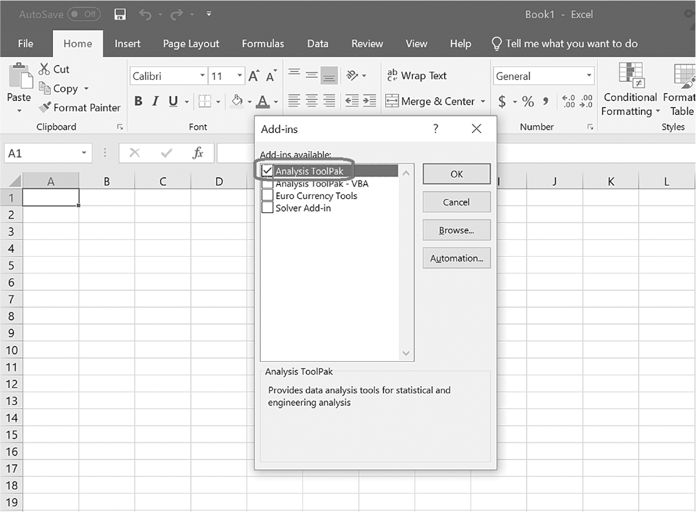
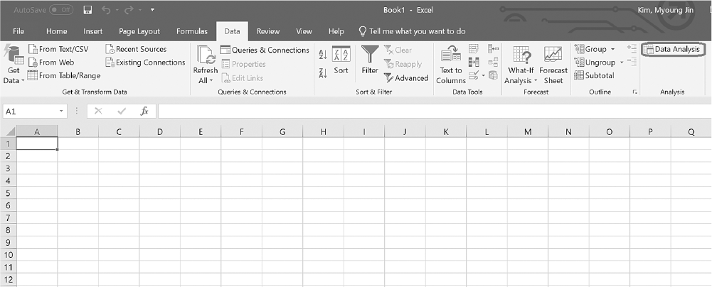
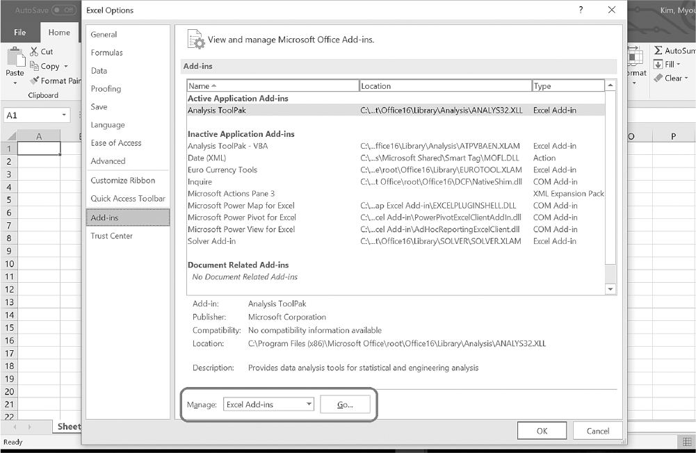
In order to explain how to analyze the data in Microsoft Excel, we will first explain how to enable and use the Data Analysis ToolPak. Go to File > Options, as displayed in Figure 7-2. Then, click on the "Add-In" category, select "Excel Add-Ins" in the Manage box, and click "Go," as displayed in Figure 7-3. Next, check the Analysis ToolPak check box in the Add-Ins box and then click "OK" (Figure 7-4). Now you should notice the "Data Analysis" ToolPak under the Data pull-down menu (Figure 7-5).

Selecting the option in Excel.

A screenshot shows a window with the Options tab in Excel highlighted.

The top right corner of the window reads, Book 1 - Excel. A list of options is displayed one below the other on the left side of the window. The options include Info, New, Open, Save, Save As, Print, Share, Export, Publish, and Close, followed by a separator and then by the options, Account, Feedback, and Options. Open is selected, and Options is marked with a rectangle surrounding it. On selection of Open, Workbooks and folders commands are displayed; also the list of recent workbooks, and older workbooks displayed.

Courtesy of Microsoft Excel © Microsoft 2020.

Selecting Excel Add-Ins in Excel.

A screenshot of the Excel Add-ins lists the names of the Add-ins, location, and type. Below are information on the Add-ins: name, publisher, compatibility, and description, like, provides data analysis tools for statistical ad engineering analysis.

Courtesy of Microsoft Excel © Microsoft 2020.

Selecting the Analysis ToolPak from the Add-In list in Excel.

A screenshot shows the selection of Analysis ToolPak from the list of Add-ins, with its description below—Provides data analysis tools for statistical and engineering analysis. The buttons, O k, Cancel, Browse, Automation, are on the right of list.

Courtesy of Microsoft Excel © Microsoft 2020.

Data Analysis ToolPak presented in Excel.

An Excel screenshot shows the Data Analysis ToolPak in the Analysis group under Data menu in the menu bar.

Courtesy of Microsoft Excel © Microsoft 2020.

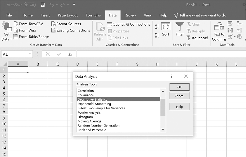
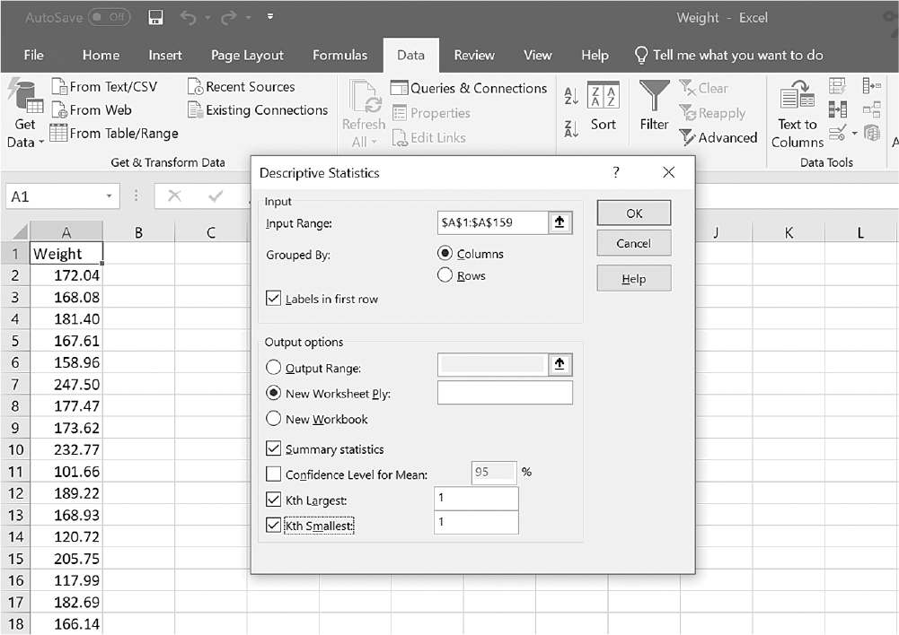
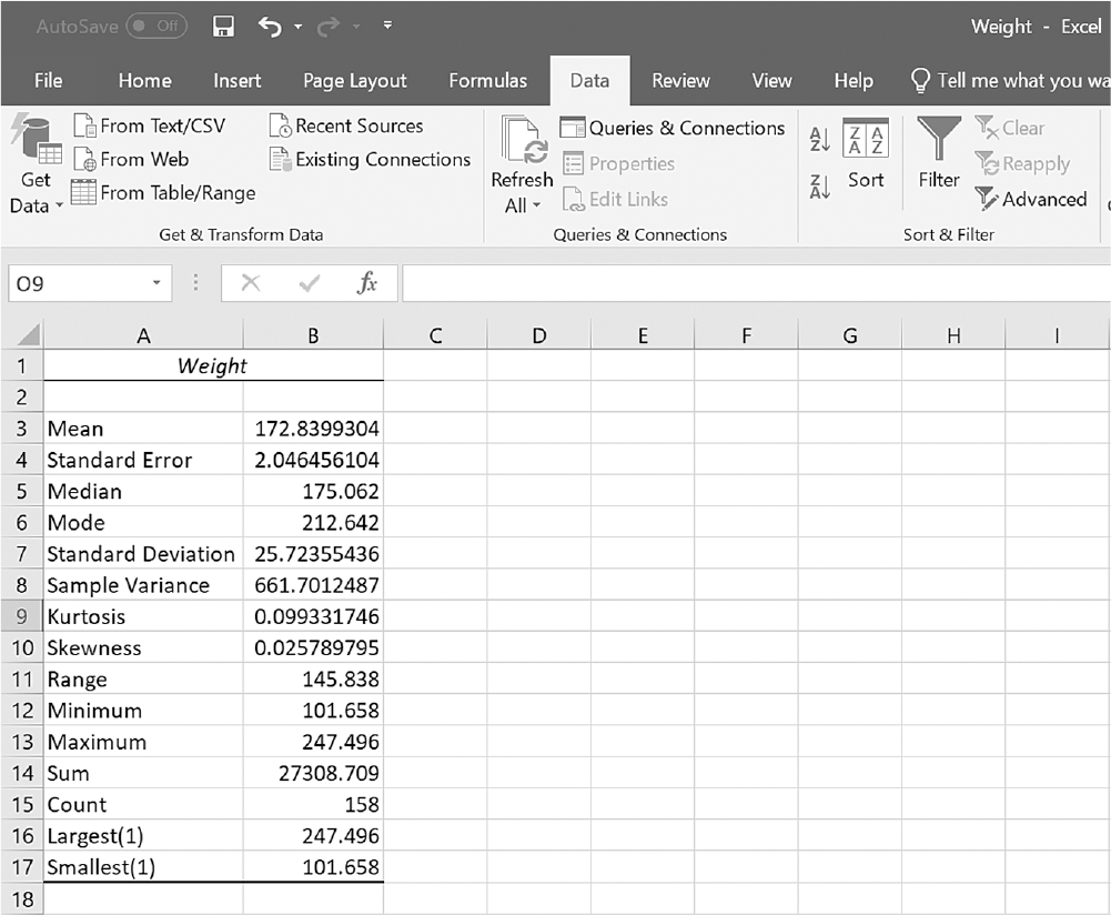
To obtain measures of central tendency in Excel, open Weight.xlsx and go to Data > Data Analysis and select "Descriptive Statistics" from the Analysis Tools list in the Data Analysis dialog box (Figure 7-6). Then, click "OK." In the Descriptive Statistics dialog box, enter A1:A159 as the Input Range, check Labels in the first row, Summary Statistics, Kth Largest, and Kth Smallest (Figure 7-7). Clicking "OK" will then produce the output, as presented in Figure 7-8.

Selecting "Descriptive Statistics" in the Data Analysis dialog box in Excel.

An Excel screenshot shows a dialog box with heading, Data Analysis, and a list of options, of which Descriptive Statistics is selected. The buttons O k, Cancel, and Help are on the right of the dialog box.

Courtesy of Microsoft Excel © Microsoft 2020.

Defining options in the Descriptive Statistics dialog box in Excel.

An Excel screenshot shows the Descriptive Statistics dialog box with fields to define data. The data in the worksheet has the column heading, Weight, with a list of numerical data.

The dialog box has two textboxes. The first textbox with heading, Input, consists of a drop-down list, input range; Grouped by with two options, Columns and Rows, preceded by option buttons; and the text, Labels in first row, preceded by a check box which is selected. The second textbox with heading, Output options, consists of a drop-down list, output range; new worksheet ply which is checked; the text summary statistics, preceded by a check box which is selected; the text confidence level for mean, preceded by an unchecked check box; the text K th largest with value 1 in the entry field, preceded by a check box which is selected; and the text K th smallest with value 1 in the entry field, preceded by a check box which is selected. The buttons, O k, Cancel, and Help, are on the right of the dialog box.

Courtesy of Microsoft Excel © Microsoft 2020.

Example output of descriptive statistics in Excel.

An Excel screenshot shows the output of weight from the descriptive statistics.

The data shows the column heading, Weight, spanning along two columns. The row entries are as follows. Row 3. Mean: 172.8399304; Standard Error: 2.046456104; Median: 175.062; Mode: 212.642; Standard Deviation: 25.72355436; Sample Variance: 661.7012487; Kurtosis: 0.099331746; Skewness: 0.025789795; Range: 145.838; Minimum: 101.658; Maximum: 247.496; Sum: 27308.709; Count: 158; Largest, 1: 247.496; Smallest, 1: 101.658.

Courtesy of Microsoft Excel © Microsoft 2020.

Obtaining Measures of Central Tendency and Variability in IBM SPSS

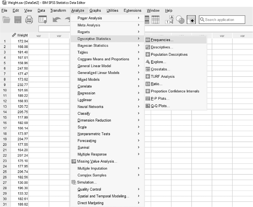
There are several places in SPSS where you can request measures of central tendency and variability. To obtain these measures, open Weight.sav and go to Analyze > Descriptive Statistics. In the next menu, choose "Frequencies" (Figure 7-9).

Selecting the frequencies window in SPSS.

A screenshot displays a dialog box with analysis options, and the frequencies option is highlighted for selection.

Reprint Courtesy of International Business Machines Corporation, © International Business Machines Corporation. "IBM SPSS Statistics software ("SPSS")". IBM®, the IBM logo, ibm.com, and SPSS are trademarks or registered trademarks of International Business Machines Corporation.

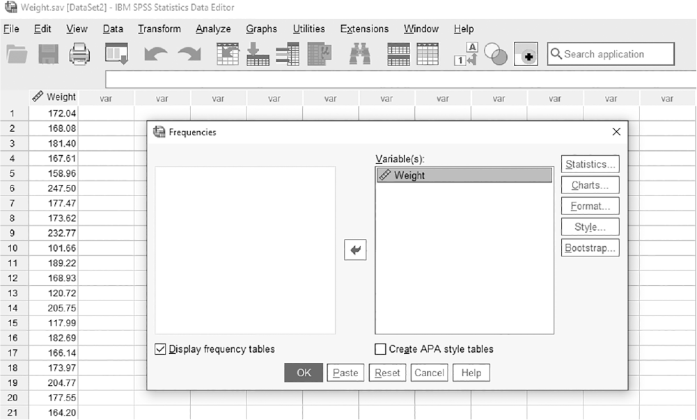
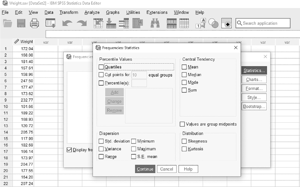
Move the variable(s) of interest, as presented in Figure 7-10. Of the five buttons on the right side of the window, select "Statistics" (Figure 7-11). You can select measures of both central tendency and variability to obtain the measures to suit your needs.

The Frequencies window in SPSS.

A screenshot displays a dialog box listing available variables, with options to move selected variables to a separate panel for frequency analysis.

Reprint Courtesy of International Business Machines Corporation, © International Business Machines Corporation. "IBM SPSS Statistics software ("SPSS")". IBM®, the IBM logo, ibm.com, and SPSS are trademarks or registered trademarks of International Business Machines Corporation.

The "Statistics" button in the Frequencies window.

A screenshot displays the Frequencies dialog box with a button labeled Statistics positioned below the variable selection panel.

Reprint Courtesy of International Business Machines Corporation, © International Business Machines Corporation. "IBM SPSS Statistics software ("SPSS")". IBM®, the IBM logo, ibm.com, and SPSS are trademarks or registered trademarks of International Business Machines Corporation.

The same measures can be obtained by choosing "Descriptives" or "Explore" under the Analyze > Descriptive Statistics drop-down menu. Note also that these measures of central tendency and variability can be obtained within windows for several other statistical procedures.

Normal Distribution

Normal distribution, a type of continuous probability distribution for a random variable, is a fundamental concept in statistics and nursing where understanding data and its patterns is crucial for making informed decisions. When a distribution is normal, the distribution is symmetrical, and the area on both sides of the distribution from the mean is equal; in other words, 50% of the data values in the set are smaller than the mean, and the other 50% are larger than the mean. Descriptive statistics help us understand whether the distribution of a continuously measured variable is normal. Figure 7-12 is an example of a normal distribution of a variable, age. In a normal distribution, the mean is located at the highest peak of the distribution, and the spread of a normal distribution can be presented in terms of the standard deviation.

Histogram with the overlying normal curve.
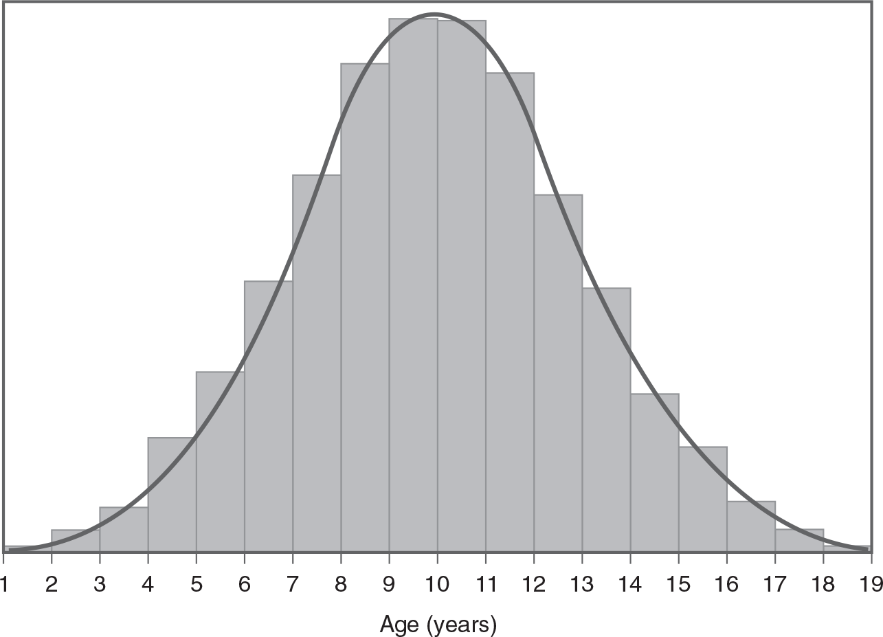
A histogram showing the age and the normal distribution are shown.

The horizontal axis of the histogram is labeled Age in years, and ranges from 1 to 19, in unit increments. The histogram increases from 1 through 9, and reaches the maximum at 9 and 10, and gradually decreases from 11 through 19. A normal curve is drawn on top of the histogram.

Why do we care about this normal distribution so much? The most important reason is that many biological and physiological variables, such as blood pressure, body temperature, and cholesterol levels, fall into an approximately normal distribution, and the measurement scores are assumed to be normally distributed when conducting most statistical analyses. Therefore, understanding normal distribution helps nurses make clinical decisions that are statistically trustworthy based on where a patient's measurements fall on this curve. We will discuss this more in Chapter 8.

Characteristics of Normal Distribution
  • It is bell-shaped and symmetrical.

  • The area under a normal curve is equal to 1.00 or 100%.

  • 68% of observations fall within one standard deviation from the mean in both directions.

  • 95% of observations fall within two standard deviations from the mean in both directions.

  • 99.7% of observations fall within three standard deviations from the mean in both directions.

  • Many normal distributions exist with different means and standard deviations.

Note that no data are ever exactly/perfectly normally distributed in reality. If so, how do we know whether a collected data set is normally distributed? We can begin with a visual display of the data in a histogram to check if the data set is normally distributed. However, a visual check alone may not be sufficient to know whether the data are normally distributed. There are statistical measures, skewness and kurtosis, which, along with a histogram, allow us to determine whether the data set is normally distributed. Skewness is a measure of whether the set is symmetrical or off-center, which means that the probabilities on both sides of the distribution are not the same. Kurtosis is a measure of how peaked a distribution is. A distribution is said to be normal when both measures of skewness and kurtosis fall within the 1 to +1 range, and nonnormal if both measures fall either below 1 or above +1. Note that these measures can be selected in the same window as measures of central tendency and variability, which we just discussed.

Figure 7-13 presents what percentage of the data set falls within how many standard deviations away from the mean. If a variable follows a normal distribution, these rules can be applied to understand the distribution of the variable in terms of the mean and the standard deviation. In addition, different normal distributions can be found when the mean and the standard deviation are defined, as presented in Figures 7-14 and 7-15.

Area under a normal distribution.
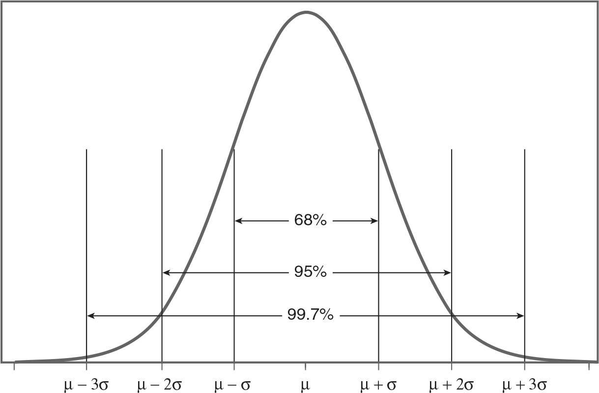
A curve shows the area under a standard normal distribution.

A standard normal distribution curve shows percentage of data falling within the standard deviations of the mean, mu. Data from the curve are as follows: 68% of data comprises mu minus epsilon and mu plus epsilon standard deviation from the mean, 95% of data comprises mu minus two times epsilon and mu plus two times epsilon standard deviation from the mean, and 99.7% of data comprises mu minus three times epsilon and mu plus three times epsilon standard deviation from the mean.

Normal distributions with different means.
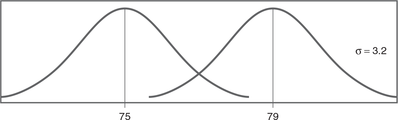
Two normal distribution curves show the mean, 75 and 79, respectively. The standard deviation equals 3.2.

Normal distributions with different standard deviations.
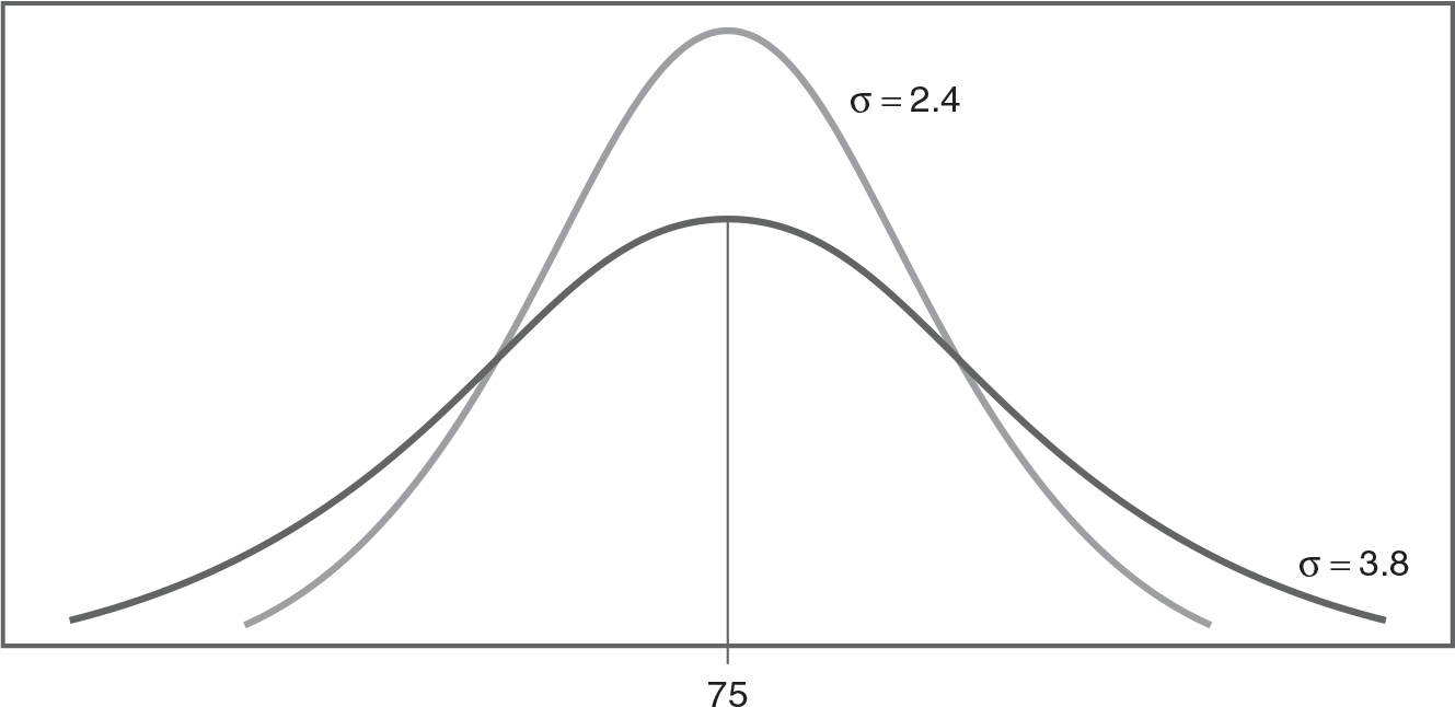
Two normal distribution curves with mean 75, show different standard deviations, 2.4 and 3.8, respectively.

We can apply the principles of the normal distribution by computing a standardized score such as a z-score. These standardized scores are useful for comparing scores computed on different scales. For example, let us consider a student who is wondering about the final exam scores in statistics and research courses. The student scored 79 out of 100 on the final exam in the statistics course and 42 out of 60 in the research course. Can the student conclude that their performance was better in statistics? Before drawing such a conclusion, the student must examine the distribution of scores on the two final exams. Let us assume that the final exam in statistics had a mean of 75 with a standard deviation of 3, and the final exam in research had a mean of 40 with a standard deviation of 2.5. The student did better than the average in both classes, but it is still difficult to judge in what course the student performed better. This question cannot be directly answered using different normal distributions because they have different means and standard deviations (i.e., they are not on an identical scale, which is necessary to make direct comparisons).

We need somehow to put these two different distributions on the same scale so that we can make a legitimate comparison of the student's performance; a standard normal distribution is the solution. By definition, a standard normal distribution is one in which all scores have been put on the same scale (standardized). These standardized scores (also known as z-scores) represent how far below or above the mean a given score falls and allow us to determine percentile/probabilities associated with a given score.

Figure 7-16 displays a graphical transition from a general normal distribution to a standard normal distribution. Characteristics of the standard normal distribution are summarized in the box on the page that follows.

Transition from a general normal distribution to a standard normal distribution.
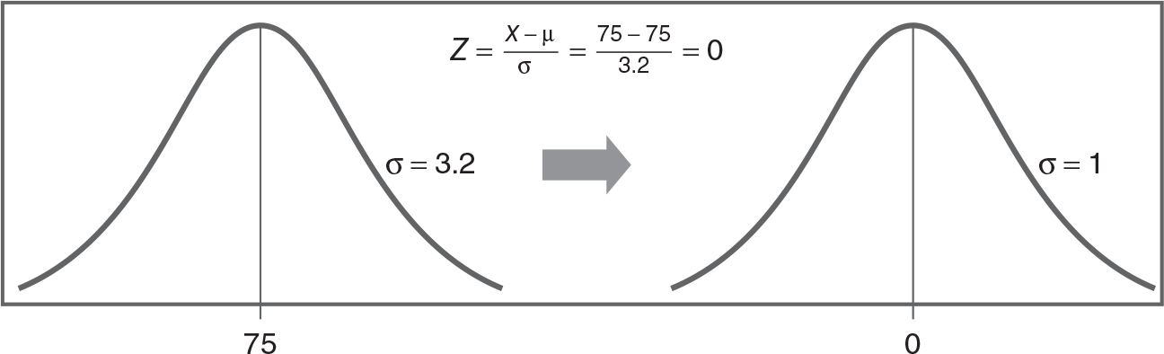
A normal distribution curve with mean 75 and standard deviation 3.2 is transitioned to a standard normal distribution curve with mean 0 and standard deviation 1. A formula reads, Z equals X minus mu, over, sigma equals 75 minus 75, over 3.2 equals 0.

To compute a z-score, you will need two pieces of information about a distribution: the mean and the standard deviation. Z-scores (standardized scores) are computed using the following equation, where the population mean (μ) is subtracted from the raw score and divided by the population standard deviation (σ). Z-scores are calculated so that positive values indicate how far a score is above the mean, and negative values indicate how far a score falls below the mean. Whether positive or negative, larger z-scores mean that scores are far away from the mean, and smaller z-scores mean that scores are close to the mean:
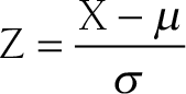
Formula reads: Z equals X minus mu over sigma.

Z-scores will be positive when a student performs better than the mean on a test (i.e., the numerator of the previous equation is positive). In contrast, z-scores will be negative when a student performs below the mean. Let us consider an example test, again a statistics final exam, with a mean of 78 and a standard deviation of 3. Suppose that Brian has a final exam score of 84. His z-score will be:
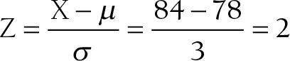
Calculation reads: Z equals X minus mu over sigma equals 84 minus 78 over 3 equals 2.

Characteristics of the Standard Normal Distribution
  • The standard normal distribution has a mean of 0 and a standard deviation of 1.

  • The area under the standard normal curve is equal to 1.00 or 100%.

  • Z-scores have associated probabilities, which are fixed and known.

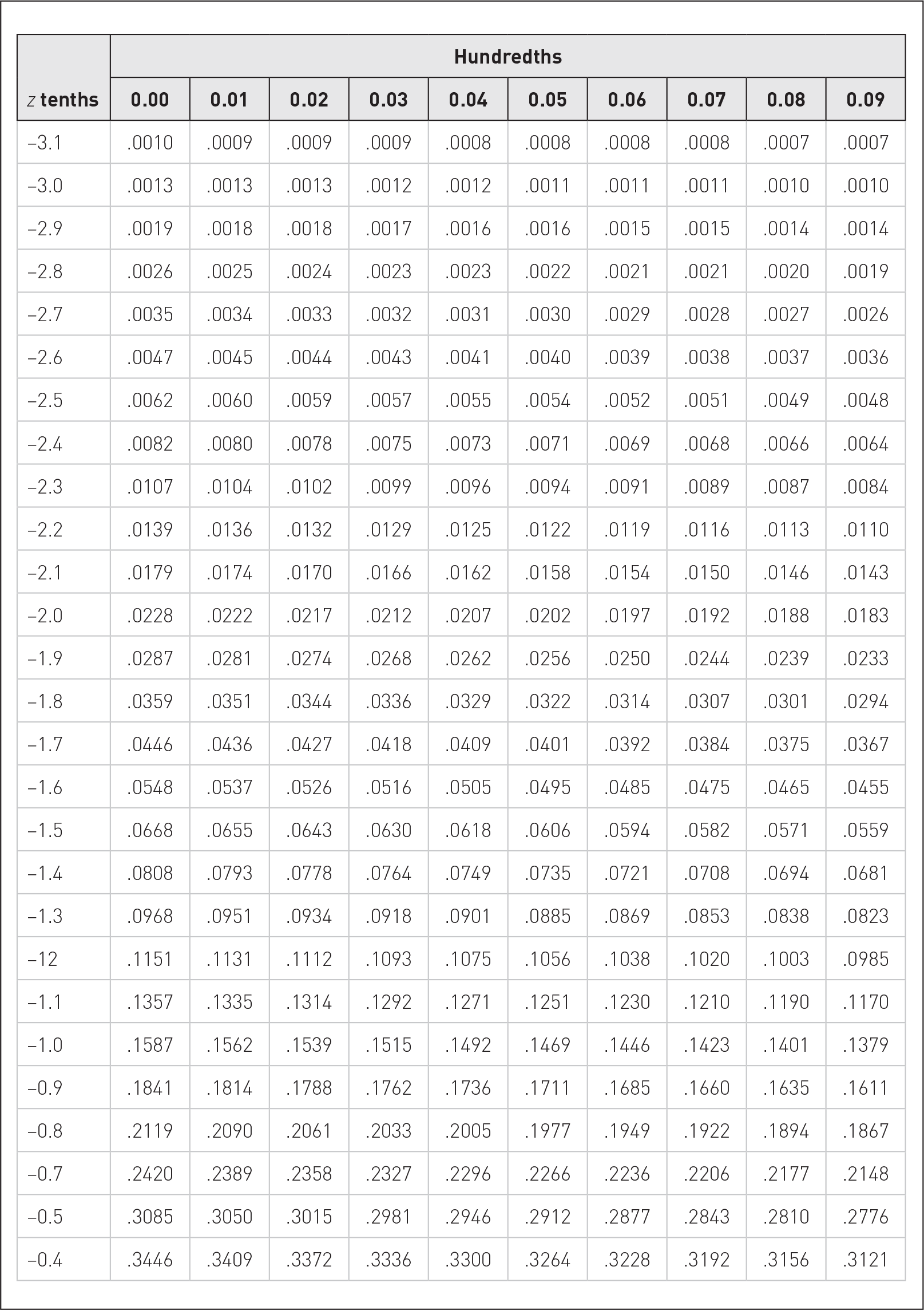
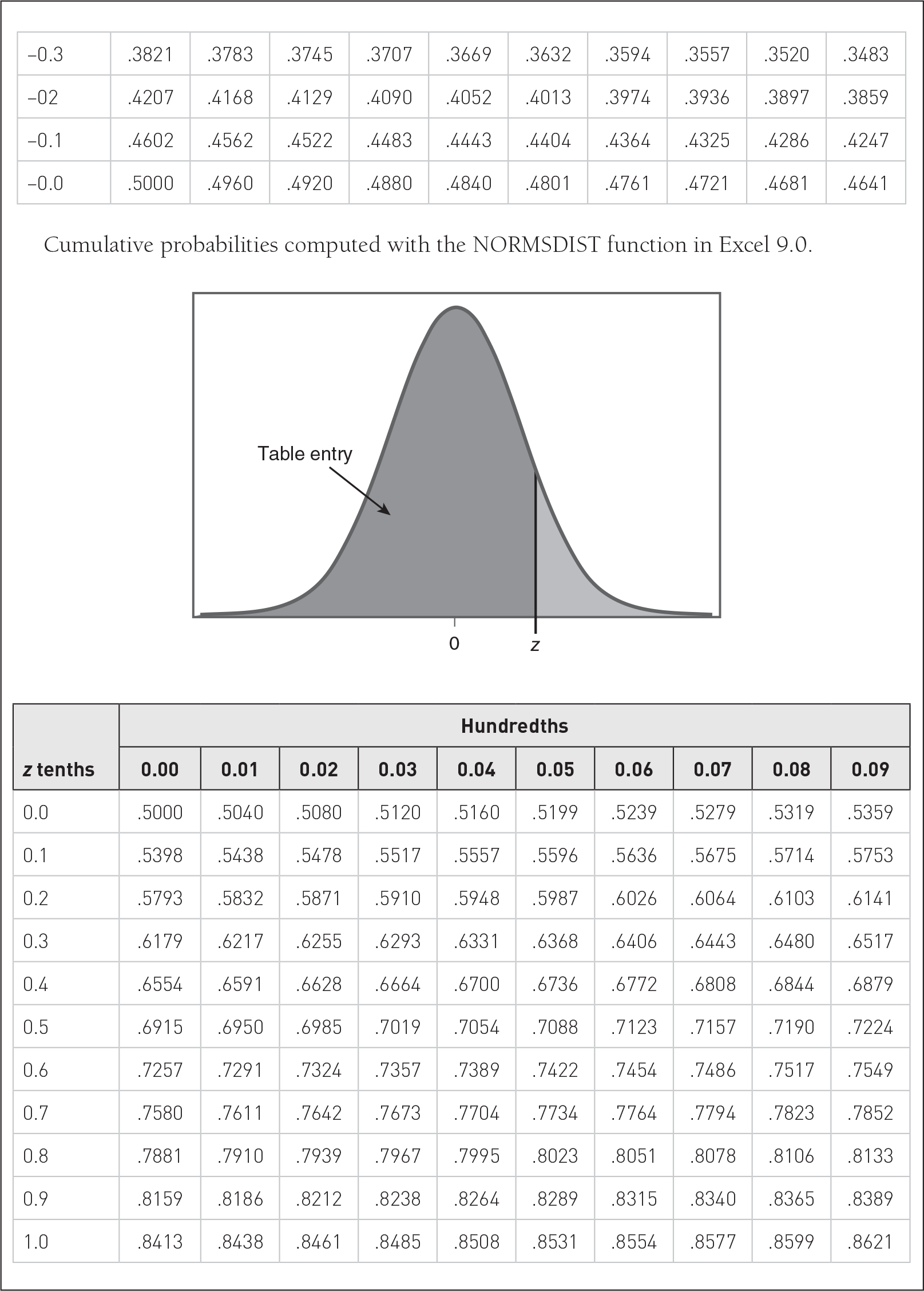
What does Brian's z-score of 2 mean in terms of his performance relative to the average person who took this statistics final exam? First, we can notice that Brian did perform better than the average person on this final exam. Second, his z-score of 2 tells us that his score is 2 standard deviations above the mean of 0 (i.e., average score of 78), because a standard normal distribution has a standard deviation of 1. However, this second point about Brian's score does not really make perfect sense to us yet. From Figure 7-17, we can notice that Brian seems to have performed better than some students in his class. However, we still do not know exactly how much better he did. To find out the exact percentile rank, we need to use a z table, as presented in Figure 7-18. Steps in using the z table to find a corresponding percentile rank are summarized in the box that follows.

Brian's z-score.
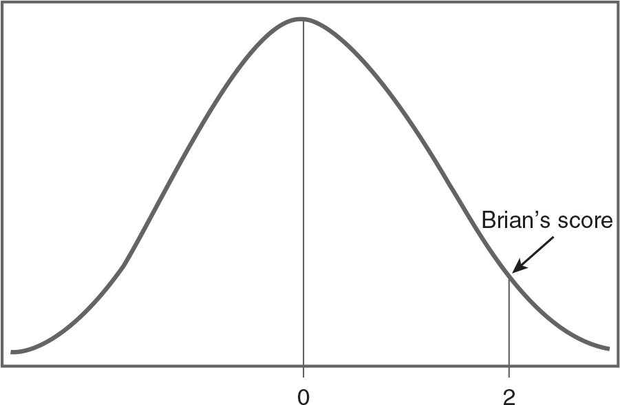
A normal distribution curve with mean 0, shows the Brian's score of 2.

z table.
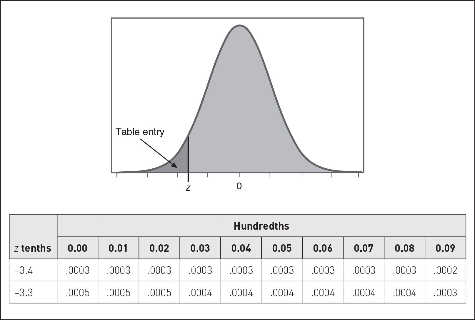
A normal distribution curve with a z table.

The curve displays the z-score below the mean, with the area under the curve up to the z-score labeled as the table entry. The table has two main columns: z tenths and z hundredths. The hundredths column is subdivided into ten subcolumns: 0.00, 0.01, 0.02, 0.03, 0.04, 0.05, 0.06, 0.07, 0.08, and 0.09. Row entries are as follows. Row 1: negative 3.4, .0003, .0003, .0003, .0003, .0003, .0003, .0003, .0003, .0003, .0002. Row 2: negative 3.3, .0005, .0005, .0005, .0004, .0004, .0004, .0004, .0004, .0004, .0003. Row 3: negative 3.2, .0007, .0007, .0006, .0006, .0006, .0006, .0006, .0005, .0005, .0005. Row 4: negative 3.1, .0010, .0009, .0009, .0009, .0008, .0008, .0008, .0008, .0007, .0007. Row 5: negative 3.0, .0013, .0013, .0013, .0012, .0012, .0011, .0011, .0011, .0010, .0010. Row 6: negative 2.9, .0019, .0018, .0018, .0017, .0016, .0016, .0015, .0015, .0014, .0014. Row 7: negative 2.8, .0026, .0025, .0024, .0023, .0023, .0022, .0021, .0021, .0020, .0019. Row 8: negative 2.7, .0035, .0034, .0033, .0032, .0031, .0030, .0029, .0028, .0027, .0026. Row 9: negative 2.6, .0047, .0045, .0044, .0043, .0041, .0040, .0039, .0038, .0037, .0036. Row 10: negative 2.5, .0062, .0060, .0059, .0057, .0055, .0054, .0052, .0051, .0049, .0048. Row 11: negative 2.4, .0082, .0080, .0078, .0075, .0073, .0071, .0069, .0068, .0066, .0064. Row 12: negative 2.3, .0107, .0104, .0102, .0099, .0096, .0094, .0091, .0089, .0087, .0084. Row 13: negative 2.2, .0139, .0136, .0132, .0129, .0125, .0122, .0119, .0116, .0113, .0110. Row 14: negative 2.1, .0179, .0174, .0170, .0166, .0162, .0158, .0154, .0150, .0146, .0143. Row 15: negative 2.0, .0228, .0222, .0217, .0212, .0207, .0202, .0197, .0192, .0188, .0183. Row 16: negative 1.9, .0287, .0281, .0274, .0268, .0262, .0256, .0250, .0244, .0239, .0233. Row 17: negative 1.8, .0359, .0351, .0344, .0336, .0329, .0322, .0314, .0307, .0301, .0294. Row 18: negative 1.7, .0446, .0436, .0427, .0418, .0409, .0401, .0392, .0384, .0375, .0367. Row 19: negative 1.6, .0548, .0537, .0526, .0516, .0505, .0495, .0485, .0475, .0465, .0455. Row 20: negative 1.5, .0668, .0655, .0643, .0630, .0618, .0606, .0594, .0582, .0571, .0559. Row 21: negative 1.4, .0808, .0793, .0778, .0764, .0749, .0735, .0721, .0708, .0694, .0681. Row 22: negative 1.3, .0968, .0951, .0934, .0918, .0901, .0885, .0869, .0853, .0838, .0823. Row 23: negative 1.2, .1151, .1131, .1112, .1093, .1075, .1056, .1038, .1020, .1003, .0985. Row 24: negative 1.1, .1357, .1335, .1314, .1292, .1271, .1251, .1230, .1210, .1190, .1170. Row 25: negative 1.0, .1587, .1562, .1539, .1515, .1492, .1469, .1446, .1423, .1401, .1379. Row 26: negative 0.9, .1841, .1814, .1788, .1762, .1736, .1711, .1685, .1660, .1635, .1611. Row 27: negative 0.8, .2119, .2090, .2061, .2033, .2005, .1977, .1949, .1922, .1894, .1867. Row 28: negative 0.7, .2420, .2389, .2358, .2327, .2296, .2266, .2236, .2206, .2177, .2148. Row 29: negative 0.6, .2743, .2709, .2676, .2643, .2611, .2578, .2546, .2514, .2483, .2451. Row 30: negative 0.5, .3085, .3050, .3015, .2981, .2946, .2912, .2877, .2843, .2810, .2776. Row 31: negative 0.4, .3446, .3409, .3372, .3336, .3300, .3264, .3228, .3192, .3156, .3121. Row 32: negative 0.3, .3821, .3783, .3745, .3707, .3669, .3632, .3594, .3557, .3520, .3483. Row 33: negative 0.2, .4207, .4168, .4129, .4090, .4052, .4013, .3974, .3936, .3897, .3859. Row 34: negative 0.1, .4602, .4562, .4522, .4483, .4443, .4404, .4364, .4325, .4286, .4247. Row 35: negative 0.0, .5000, .4960, .4920, .4880, .4840, .4801, .4761, .4721, .4681, .4641.
A normal distribution curve with a z table.

The curve displays the z-score beyond the mean, with the area under the curve up to the z-score labeled as the table entry. The table has two main columns: z tenths and z hundredths. The hundredths column is subdivided into ten subcolumns: 0.00, 0.01, 0.02, 0.03, 0.04, 0.05, 0.06, 0.07, 0.08, and 0.09. Row entries are as follows: Row 1: 0.0, .5000, .5040, .5080, .5120, .5160, .5199, .5239, .5279, .5319, .5359. Row 2: 0.1, .5398, .5438, .5478, .5517, .5557, .5596, .5636, .5675, .5714, .5753. Row 3: 0.2, .5793, .5832, .5871, .5910, .5948, .5987, .6026, .6064, .6103, .6141. Row 4: 0.3, .6179, .6217, .6255, .6293, .6331, .6368, .6406, .6443, .6480, .6517. Row 5: 0.4, .6554, .6591, .6628, .6664, .6700, .6736, .6772, .6808, .6844, .6879. Row 6: 0.5, .6915, .6950, .6985, .7019, .7054, .7088, .7123, .7157, .7190, .7224. Row 7: 0.6, .7257, .7291, .7324, .7357, .7389, .7422, .7454, .7486, .7517, .7549. Row 8: 0.7, .7580, .7611, .7642, .7673, .7704, .7734, .7764, .7794, .7823, .7852. Row 9: 0.8, .7881, .7910, .7939, .7967, .7995, .8023, .8051, .8078, .8106, .8133. Row 10: 0.9, .8159, .8186, .8212, .8238, .8264, .8289, .8315, .8340, .8365, .8389. Row 11: 1.0, .8413, .8438, .8461, .8485, .8508, .8531, .8554, .8577, .8599, .8621. Row 12: 1.1, .8643, .8665, .8686, .8708, .8729, .8749, .8770, .8790, .8810, .8830. Row 13: 1.2, .8849, .8869, .8888, .8907, .8925, .8944, .8962, .8980, .8997, .9015. Row 14: 1.3, .9032, .9049, .9066, .9082, .9099, .9115, .9131, .9147, .9162, .9177. Row 15: 1.4, .9192, .9207, .9222, .9236, .9251, .9265, .9279, .9292, .9306, .9319. Row 16: 1.5, .9332, .9345, .9357, .9370, .9382, .9394, .9406, .9418, .9429, .9441. Row 17: 1.6, .9452, .9463, .9474, .9484, .9495, .9505, .9515, .9525, .9535, .9545. Row 18: 1.7, .9554, .9564, .9573, .9582, .9591, .9599, .9608, .9616, .9625, .9633. Row 19: 1.8, .9641, .9649, .9656, .9664, .9671, .9678, .9686, .9693, .9699, .9706. Row 20: 1.9, .9713, .9719, .9726, .9732, .9738, .9744, .9750, .9756, .9761, .9767. Row 21: 2.0, .9772, .9778, .9783, .9788, .9793, .9798, .9803, .9808, .9812, .9817. Row 22: 2.1, .9821, .9826, .9830, .9834, .9838, .9842, .9846, .9850, .9854, .9857. Row 23: 2.2, .9861, .9864, .9868, .9871, .9875, .9878, .9881, .9884, .9887, .9890. Row 24: 2.3, .9893, .9896, .9898, .9901, .9904, .9906, .9909, .9911, .9913, .9916. Row 25: 2.4, .9918, .9920, .9922, .9925, .9927, .9929, .9931, .9932, .9934, .9936. Row 26: 2.5, .9938, .9940, .9941, .9943, .9945, .9946, .9948, .9949, .9951, .9952. Row 27: 2.6, .9953, .9955, .9956, .9957, .9959, .9960, .9961, .9962, .9963, .9964. Row 28: 2.7, .9965, .9966, .9967, .9968, .9969, .9970, .9971, .9972, .9973, .9974. Row 29: 2.8, .9974, .9975, .9976, .9977, .9977, .9978, .9979, .9979, .9980, .9981. Row 30: 2.9, .9981, .9982, .9982, .9983, .9984, .9984, .9985, .9985, .9986, .9986. Row 31: 3.0, .9987, .9987, .9987, .9988, .9988, .9989, .9989, .9989, .9990, .9990. Row 32: 3.1, .9990, .9991, .9991, .9991, .9992, .9992, .9992, .9992, .9993, .9993. Row 33: 3.2, .9993, .9993, .9994, .9994, .9994, .9994, .9994, .9995, .9995, .9995. Row 34: 3.3, .9995, .9995, .9995, .9996, .9996, .9996, .9996, .9996, .9996, .9997. Row 35: 3.4, .9997, .9997, .9997, .9997, .9997, .9997, .9997, .9997, .9997, .9998. Text above the table reads: Cumulative probabilities computed with the NORMSDIST function in Excel 9.0.
A normal distribution curve with a z table.
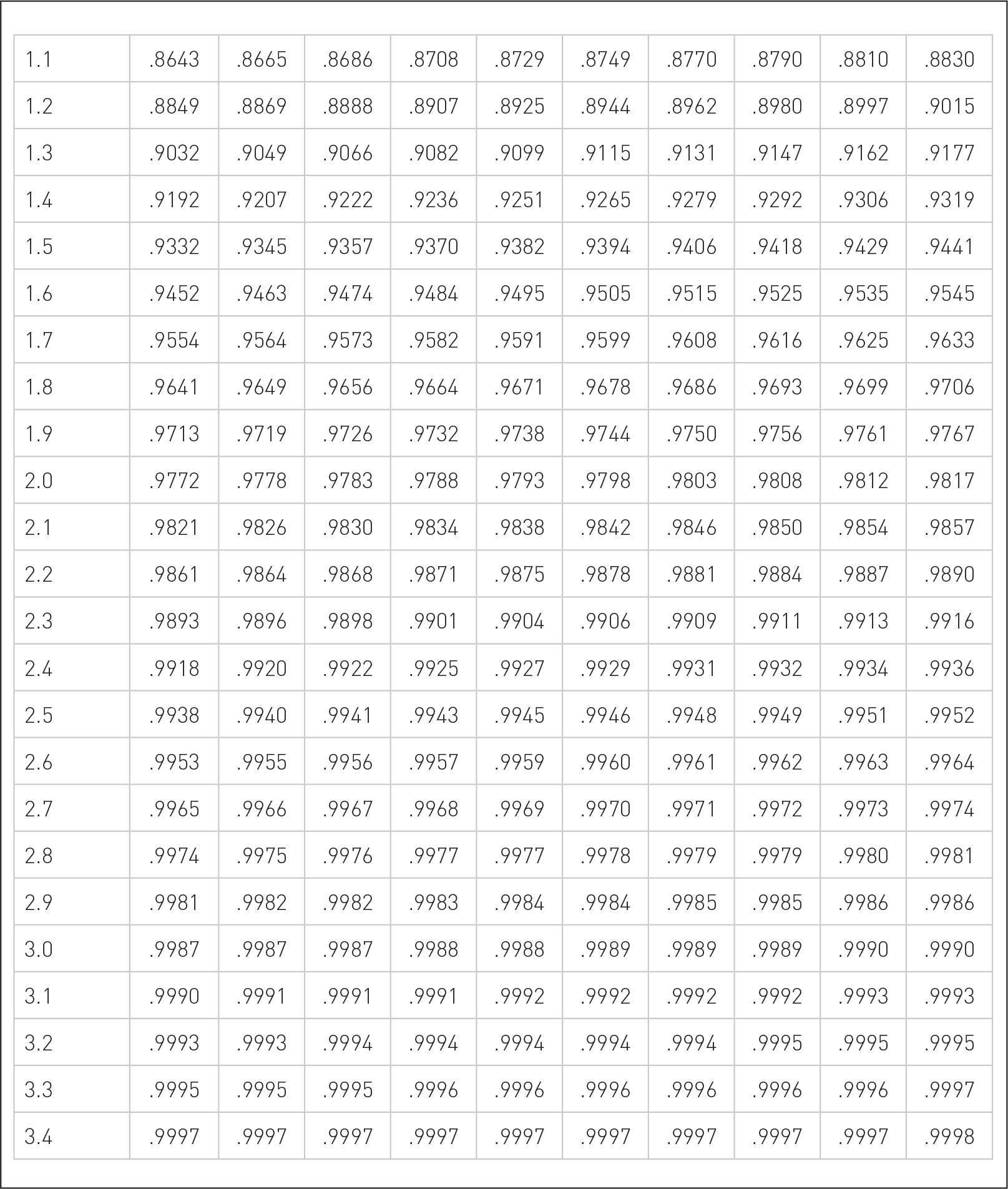
A normal distribution curve with a z table.

Using the z Table to Find a Corresponding Percentile Rank of a Score
  1. Convert Brian's final exam score to a corresponding z-score.

  2. Locate the row in the z table for a z-score of +2.00. Note that the z-scores in the first column are shown to only the first decimal place. Also, locate the column for 0.00 so that you get 2.00 when you add 2.0 and 0.00.

  3. Brian's z-score of +2.00 gives probability of 0.9772 to the left.

  4. Therefore, Brian's final exam score of +2.00 corresponds to the 98th percentile. Brian did better than 98% of the students in the class.

Let us consider another example that will help us understand how to find the corresponding probability for a given score. The sodium intakes for a group of cardiac rehabilitation patients are known to have a mean of 4,500 mg/day and a standard deviation of ±150 mg/day. Assuming that the sodium intake is normally distributed, let us find the probability that a randomly selected patient will have a sodium intake level below 4,275 mg/day. First, we need to convert this value into the z-score. The corresponding z-score for 4,275 mg/day will be:

Calculation reads: Z equals X minus mu over sigma equals 4,275 minus 4,500 over 150 equals negative 1.5.

Locating the row in the z table for a z-score of 1.5 and the column for 0.00, you should get a probability of 0.0668. Therefore, the probability that a randomly selected patient will have a sodium intake below 4,275 mg/ day will be 6.68%. How about the probability that a randomly selected patient will have between 4,350 mg/day and 4,725 mg/day? Notice here that we have two scores to transform. The corresponding z-score of the lower level, 4,350 mg/day, will be:

Calculation reads: Z equals X minus mu over sigma equals 4,350 minus 4,500 over 150 equals negative 1.

and the upper level, 4,725 mg/day, will be

Calculation reads: Z equals X minus mu over sigma equals 4,725 minus 4,500 over 150 equals positive 1.5.

Therefore, we are considering the area under the normal curve between 1 and +1.5 standard deviations, as presented in Figure 7-19. The probability to the left of +1.5 is 0.9332, and the probability to the left of 1 is 0.1587. To get the probability between 1 and +1.5, we will subtract 0.1587 from 0.9332 and should get 0.7745. Therefore, the probability that a randomly selected patient will have a sodium intake between 4,350 mg/day and 4,725 mg/day will be 77.45%. Finding the corresponding probabilities for a given score can be tricky, so we recommend that you work on as many examples as you can, including what is provided at the end of this chapter.

The normal curve between -1 and +1.5 standard deviations.
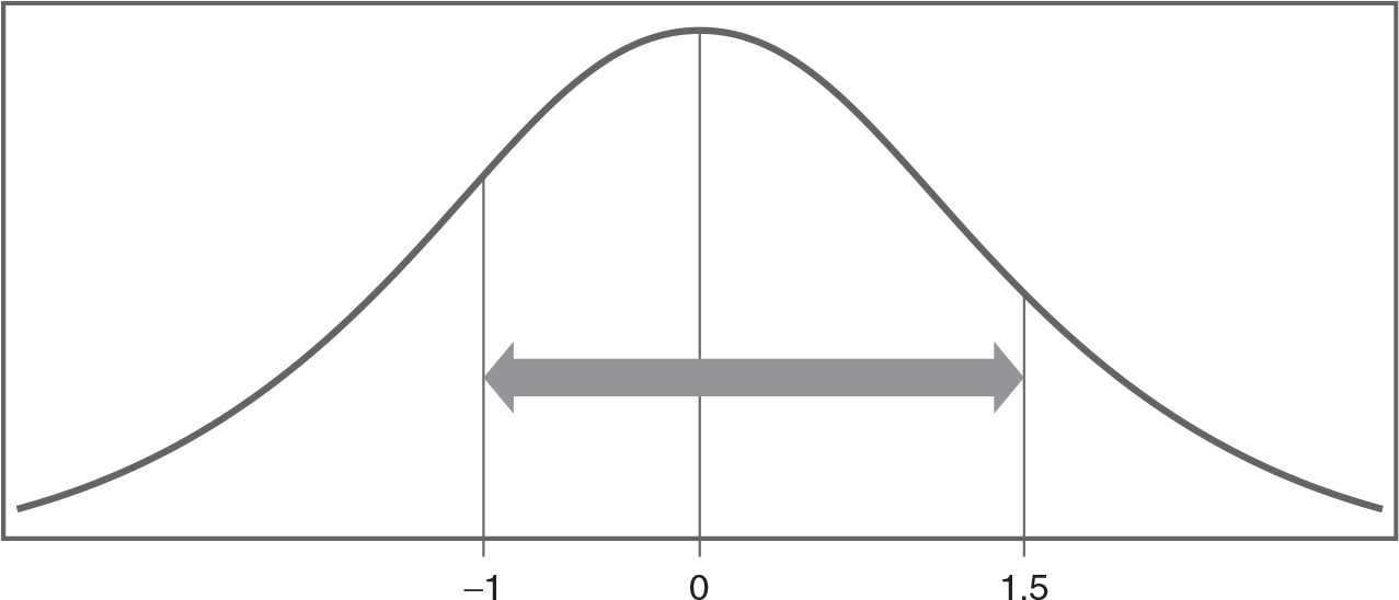
A standard normal distribution curve is shown between the standard deviations, minus 1 and plus 1.5, from the mean.

As a closing note about the standard normal distribution, recall that the following are true when a variable is normally distributed:

  • 68% of observations fall within one standard deviation from the mean in both directions.

  • 95% of observations fall within two standard deviations from the mean in both directions.

  • 99.7% of observations fall within three standard deviations from the mean in both directions.

This means that 68% of the z-scores will fall between 1 and +1, 95% of the z-scores will fall between 2 and +2, and 99.7% of the z-scores will fall between 3 and +3 because the standard normal distribution has a mean of 0 and a standard deviation of 1. This is important because any z-score that is greater than +3 or less than 3 can be treated as unusual.
Confidence Interval

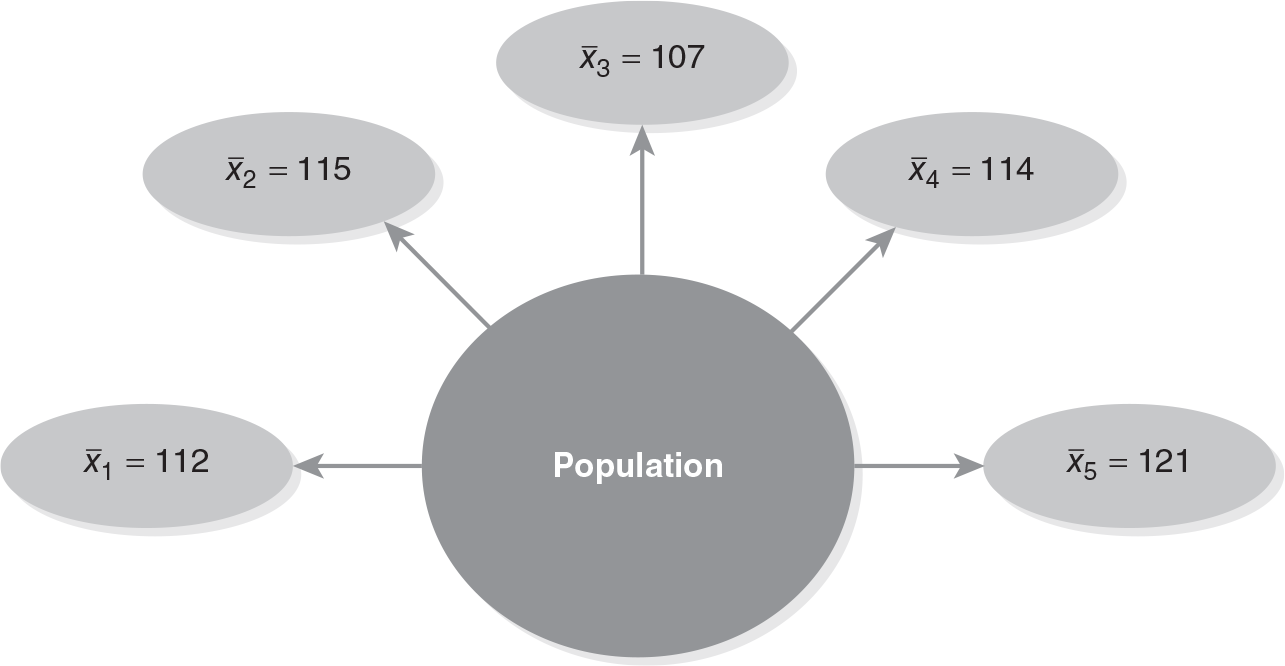
Up to this point, all of the estimates we have calculated were with a single number. Measures of both central tendency and variability were a single number, which allowed us to say that those measures were the average measurements and the spread of values on the average of a given variable, respectively. These are called point estimates. However, we may not be lucky enough to hit exactly or even close to the actual average in the population, because we are likely to use a sample taken from the population. In other words, we will never be sure that our estimates will accurately reflect values in the population as a whole, as presented in Figure 7-20.

Different sample means from a population.

A diagram illustrates sampling means, with population, and four sample means, X bar, equaling 112, 115, 107, 114, and 121, respectively.

To deal with this problem, we can create boundaries, or a range of estimates within which we can be reasonably sure the true population parameter lies, instead of computing a single estimate from a sample; these boundaries are called confidence intervals. It is another way of answering an important question, "How well does the sample statistic represent the unknown population parameter?"

Confidence intervals use confidence levels in the computation. The confidence level is a statistical concept that represents the degree of certainty or probability that a confidence interval contains the true population parameter. It is determined by the researcher and reflects how accurate you want to be in computing a confidence interval as a percentage. There are three confidence levels that you can choose from: 90%, 95%, and 99% (although the 95% confidence level seems to be the most popular choice). What does confidence interval mean? Let us say that you chose a 95% confidence level to compute a confidence interval; this means that if you were to hypothetically compute 100 confidence intervals, 95 of those confidence intervals will contain the population parameter and 5 of those will not. Another way of thinking about it is to say that should we calculate 100 confidence intervals, 5 of those would likely not be accurate. There are different equations for different parameters in the computation of confidence intervals, but we will introduce only one here for a population mean and focus on how to interpret the computed confidence interval.

Let us assume that you are a nurse educator and want to investigate the average number of hours that nursing students at a local university spend per week studying statistics. The number of hours is measured on the ratio level of measurement, and we are considering the mean hours. Because we need to compute a confidence interval for the mean, we will use the following equation:

Formula reads: x-bar minus Z subscript open parenthesis alpha over 2 close parenthesis times S over square root of n less than mu less than x-bar plus Z subscript open parenthesis alpha over 2 close parenthesis times S over square root of n.

where

is the sample mean; zα/2 is the corresponding z-value for α/2, where α is equal to 1 confidence level; s is the sample standard deviation; and n is the sample size.

Let us assume that we obtained a sample of 30 nursing students and the distribution of the number of hours that they study for statistics per week had a mean of 8 and standard deviation of 2. We want to compute a 90% confidence interval where zα/2 = 1.645. Our α is .10 because we are using a 90% confidence level and α/2 is .05. We will find that the corresponding z-score for the closest probability to .95 (1 .05) inside the z table is 1.64, 1.65, or 1.645 (with the middle value between 1.64 and 1.65, as we cannot find the exact probability). Using 1.645, the 90% confidence interval will be:

Calculation reads: 8 minus 1.645 times open parenthesis 2 over square root of 30 close parenthesis less than mu less than 8 plus 1.645 times open parenthesis 2 over square root of 30 close parenthesis.

7.3993 <μ< 8.6007

We can conclude from this finding that 90% of the time, the mean will fall between 7.40 and 8.60 hours of studying for statistics.

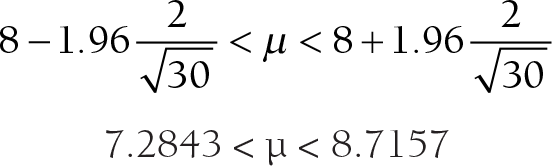
Consider now that you want to compute a 95% confidence interval for the same example that we previously used. Our zα/2 is 1.96 because our α/2 is .025 for a 95% confidence level, and the 95% confidence interval will be:

Calculation reads: Line 1: 8 minus 1.96 times open parenthesis 2 over square root of 30 close parenthesis less than mu less than 8 plus 1.96 times open parenthesis 2 over square root of 30 close parenthesis. Line 2: 7.2843 less than mu less than 8.7157.

In this case, we can conclude that 95% of the time, the mean hours of studying for statistics fall between 7.28 and 8.72.

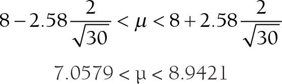
How about a 99% confidence interval for the same example? Our zα/2 is 2.58 because our α/2 is .005 for a 99% confidence level, and the 99% confidence interval will be:

Calculation reads: Line 1: 8 minus 2.58 times open parenthesis 2 over square root of 30 close parenthesis less than mu less than 8 plus 2.58 times open parenthesis 2 over square root of 30 close parenthesis. Line 2: 7.0579 less than mu less than 8.9421.

In this example, we can conclude that 99% of the time, the mean hours that students spend studying statistics is between 7.06 and 8.94.

As you observe these three confidence intervals, you will notice that the confidence interval gets wider as your desired confidence level increases. This makes sense because the wider the confidence interval, the more you can be sure that the interval will include the population parameter.

Summary

Descriptive statistics, such as measures of central tendency and variability, help us understand typical cases in a sample and the distribution of values in a data set more clearly. Measures of central tendency include mode, median, and mean, which provide us with an idea of the typical/average data value in the data set. The mode should be used only for categorical data, as it basically counts frequency. Because the median is less sensitive to unusual data values, it should be reported when an unusual data value is present in the data set. Otherwise, the mean should be reported, as it possesses statistically preferable characteristics. Measures of variability include the range, the interquartile range, the variance, and the standard deviation, and these convey the spread of values and give us an idea of the accuracy of the measures of central tendency. The range should be used as a crude measure of variability, as it is extremely sensitive to the presence of unusual data values. The interquartile range should be reported when an unusual or outlying data value is present in the data set. Otherwise, the standard deviation should be reported, as it possesses statistically preferable characteristics.

A normal distribution is an important probability distribution that can represent many human characteristics, such as height, weight, and blood pressure. Skewness and kurtosis can be used to assess whether a variable is normally distributed; values should be between 1 and +1 in order to be normal. It is important that variables of interest be normally distributed, as most statistical analyses assume a normal distribution.

When a variable is normally distributed, 68% of observations will fall within one standard deviation from the mean, 95% of observations will fall within two standard deviations from the mean, and 99.7% of observations will fall within three standard deviations from the mean. Any value that falls outside of the three standard deviations can be treated as an unusual value for the data set.

Z-scores are a good example of how we can compute standardized scores to determine where any given score falls in a normal distribution. We can use standardized scores to make comparisons of a single score, such as on a standardized test, with all other scores.

Instead of estimating an unknown population parameter with a single number or point estimate, we can compute an interval, called a confidence interval, as a different way of answering the question, "How well does the sample statistic represent an unknown population parameter?" Confidence intervals are interpreted as the interval that will include the true parameter with a given confidence level, either 90%, 95%, or 99%. As the percentage of the confidence level goes up (i.e., increased confidence that the mean falls within that range), the likelihood of the confidence interval including a true population parameter increases.

Critical Thinking Questions

  1. What is the purpose of computing descriptive statistics? Why should we include these with visual displays of a data set?

  2. Which measure of central tendency and variability should be reported when an unusual data value is present in the data set? Why?

  3. The 95% confidence interval for sodium content level in 32 nursing home patients is (4,250 mg/day, 4,750 mg/day). What does this confidence interval tell us?

  4. How would you explain the importance of selecting the appropriate measure of central tendency (mean, median, mode) when analyzing patient outcomes? Provide an example where the mean might be misleading.

  5. In a study comparing two groups, one receiving a new treatment and the other a standard treatment, the mean recovery time is the same, but the standard deviations differ significantly. How would you interpret this finding?

  6. Describe a situation in which the range of a data set could be misleading in the context of nursing research. What other measures of spread would you use to complement the range?

  7. How would you explain the significance of using z-scores in comparing individual patient data points to the overall population in a clinical study?

  8. How could the concept of variance be applied to understanding differences in patient recovery times? What might high variance indicate about the treatment's effectiveness?

Self-Quiz

  1. Which measure of central tendency is most appropriate when the data is skewed?

    1. Mean

    2. Median

    3. Mode

    4. Range

  2. True or False: The standard deviation can be negative.

  3. True or False: Descriptive statistics are used to summarize the characteristics of the sample and the measures in the data set.

  4. True or False: The variance in length of stay at a local hospital is 25. The standard deviation is 5, and this is how each value differs on average from the mean.

  5. Which of the following is not a measure of central tendency?

    1. Mode

    2. Interquartile range

    3. Mean

    4. Median

  6. In a normal distribution, what is the probability that a value falls within one standard deviation of the mean?

    1. 50%

    2. 90%

    3. 68%

    4. 99%

  7. Find the area under the normal distribution curve in the following locations:

    1. To the left of z = 0.59

    2. To the left of z = 2.41

    3. To the right of z = 1.32

    4. To the right of z = 0.27

    5. Between 0.87 and 0.87

    6. Between 2.99 and 1.34

  8. The average time it takes for emergency nurses to respond to an emergency call is known to be 3 minutes. Assume the variable is approximately normally distributed, and the standard deviation is 1 minute. If we randomly select an emergency nurse, find the probability of the selected nurse responding to an emergency call in less than 2 minutes.

  9. Twenty-five local nursing home residents have an average age of 72, and the standard deviation is 8. The director of the nursing home wants to compute a 95% confidence interval to understand the accuracy of an estimate for the average age of all residents. What is the 95% confidence interval?

    1. (65.23, 78.77)

    2. (68.86, 75.14)

    3. (65.00, 74.00)

    4. (62.86, 82.14)

  10. True or False: The interquartile range (IQR) measures the range of the middle 50% of data points in a data set.

Reference

HuaC. L., SmithL., ZimmermanS., GadkariG., CarderP., SloaneP. D., WretmanC. J., & ThomasK. S. (2024). Admission and discharge practices among assisted living communities: The role of state regulations and organizational characteristics. The Gerontologist, 64(8). https://doi.org/10.1093/geront/gnae076McCannR., RichardsonE., SchislerE. D., SudduthA., & DobbsP. D. (2024). Cigarette and e-cigarette harm perceptions during pregnancy. Nursing Research, 73(4), 286-293. https://doi.org/10.1097/NNR.0000000000000742PillemerK., TeresiJ. A., RamirezM., EimickeJ., SilverS., BoratgisG., MeadorR., SchultzL., KongJ., Ocepek-WeliksonK., ChangE., & LachsM. (2024). Estimated prevalence of resident-to-resident aggression in assisted living. JAMA Network Open, 7(5), e249668. https://doi.org/10.1001/jamanetworkopen.2024.9668