Hypothesis Testing

Suppose that we are interested in studying whether a newly developed intervention for fall prevention is more effective in reducing fall rates than an existing approach. The question is, "How do we determine the effect of the new fall prevention intervention compared with an existing one?" We say that there is an effect when changes in one variable cause another variable to change. Recall that in intervention or experimental studies, the investigator manipulates the independent variable and then measures change in the dependent variable to determine if an effect is present and the strength of that effect. To determine whether the new intervention has an effect on fall incidence, we need to determine if the observed difference between fall rates using the existing and new interventions is meaningful and not just because of chance. Hypothesis testing is the term we use for the process of determining if an effect, association, or difference is because of chance.

In a more familiar sense, nurses use hypotheses, or informed speculations, routinely in our day-to-day work. We might ask ourselves a question such as, "I wonder if Mr. Garcia's low blood pressure is because of a change in medication or a fluid volume deficit?" We then collect data that help us establish the underlying cause of the low blood pressure and respond appropriately to manage the problem.

Hypothesis testing in the world of evidence-based practice and research is also about addressing problems, but instead of focusing on decisions for a single patient, we are interested in results that may be applied to a hypothetical average patient drawn from a sample. Hypothesis testing provides a better understanding of how much confidence we can have in the results of a study; that is, we can estimate the probability that the results are true. In research and evidence-based practice, knowing about the application of results to an average patient or population and our confidence in the results allows us to estimate the generalizability or applicability of results from any given study. Remember that generalizability is the extent to which findings from a sample may be applied to the population beyond specific conditions of the study (because of the impracticability of studying an entire population on most occasions). In other words, it is about whether the findings from a sample can be reliably extrapolated to the larger population. Because a sample is used to make inferences about the population, there will be a chance of making errors. Hypothesis testing is the foundation for making informed decisions about the strength of evidence for clinical practices.

There are five general steps in hypothesis testing based on recommendations from the American Statistical Association (ASA) (Wasserstein et al., 2019) and the International Journal of Nursing Studies (Hayat et al., 2019). Recommendations from these organizations state that investigators should quantify evidence against the null hypothesis with a p-value without dichotomizing the results using the phrases "statistically significant" and "statistically nonsignificant." Although you will likely continue to find these terms in study reports, we expect more investigators to discuss the statistical meaningfulness of hypothesis testing.

General Steps in Hypothesis Testing

State the null and alternative hypotheses.
Propose an appropriate statistical test.
Check assumptions of the chosen test.
Compute the test statistics (find the p-value).
Use the p-value to quantify evidence against the null hypothesis.

General Steps in Hypothesis Testing ⬆ ⬇

Step 1: State the Null and Alternative Hypotheses

In every study and many evidence-based practice projects, two hypotheses are formulated: the null hypothesis and the alternative hypothesis. These are competing statements.

The null hypothesis is the hypothesis that assumes there are no effects and is denoted as H₀. We usually think of the null hypothesis as an objective starting point or the center of a fulcrum, where there is no statistically discernible difference. Continuing with our falls example, we would write, "On average, there is no difference in falls between a newly developed intervention and an existing practice." In research and evidence-based practice, we design our studies to test the null hypothesis, aiming to determine whether sufficient evidence exists to reject this hypothesis in favor of the alternative hypothesis.

The alternative hypothesis, in contrast, is a hypothesis that states an effect, relationship, or difference between variables and is denoted as H₁ or H_a; it represents what we really want to know. We may write, "On average, the newly developed intervention and an existing practice have different effects on falls," or "The newly developed intervention has a better effect, on average, than that of an existing practice for preventing falls."

Step 2: Propose an Appropriate Statistical Test

Once both hypotheses have been formulated, we will decide what statistical test is best for testing the proposed hypotheses. Each statistical test has its own requirements with regard to how many variables are being measured and at what level of measurement each of these is measured. Table 8-1 briefly summarizes the key points in selecting an appropriate statistical test.

Table 8-1 Number of Variables and Level of Measurement in Choosing a Statistical Test

Independent Variables (IVs)	Dependent Variables	Statistical Tests
0 IV	Interval and ratio Categorical	One-sample t-test χ² test of goodness of fit
1 categorical IV with 2 levels (independent)	Interval and ratio	Independent t-test
	Ordinal or interval	Wilcoxon/Mann-Whitney test
	Categorical	χ²/Fisher's exact test
1 categorical IV with 2 levels (dependent)	Interval and ratio	Dependent t-test
	Ordinal or interval	Wilcoxon signed rank test
	Categorical	McNemar test
1 categorical IV with more than 2 levels (independent)	Interval and ratio	One-way analysis of variance (ANOVA)
1 categorical IV with more than 2 levels (independent)	Ordinal or interval	Kruskal-Wallis test
1 categorical IV with more than 2 levels (dependent)	Interval and ratio	One-way repeated measures ANOVA
	Ordinal or interval	Friedman test
	Categorical	Repeated measures logistic regression
2 or more categorical IVs (independent)	Interval and ratio	Factorial ANOVA
2 or more categorical IVs (independent)	Categorical	Factorial logistic regression
1 interval IV	Interval and ratio Ordinal or interval Categorical	Correlation (Pearson's)/simple linear regression Nonparametric correlation (Spearman's rho) Simple logistic regression
1 or more interval IVs and/or 1 or more categorical IVs	Interval and ratio Categorical	Multiple regression/analysis of covariance (ANCOVA) Logistic regression/discriminant analysis

Determining the type of research design, number of variables in the research question and/or hypotheses, and levels of measurement of variables in those hypotheses is critical in the research process. Let us consider an example null hypothesis: There is no relationship between weight and systolic blood pressure (SBP). We are analyzing a relationship between two variables, weight and SBP, and both are measured on the ratio level of measurements. Table 8-1 shows this is a perfect hypothesis for using Pearson's correlation coefficient. Note that we should use a nonparametric correlation coefficient, such as Spearman's rho, if one of the variables is measured on the ordinal level of measurement.

Step 3: Check Assumptions of the Chosen Test

Once the investigator selects a statistical test that is best for the proposed hypotheses, the assumptions of that test must be scrutinized to ensure that the results are trustworthy. Each statistical test, such as Pearson's correlation coefficient, will have unique assumptions, but there are some common assumptions across tests. These include normality (the distribution of data values follows a normal curve), equal variance across groups (the variances across groups are equal), and independence (that there is no overlap of members between groups). The details of these common assumptions will be covered in Chapter 9.

Step 4: Compute the Test Statistics (Find the p-Value)

As we proceed in this text, we will discuss each test and how to select the necessary options in both Microsoft Excel and IBM SPSS Statistics software (SPSS). Note that the test statistic from running the proposed test will determine the p-value, which can be used to quantify evidence against the null hypothesis.

Step 5: Use the p-Value to Quantify Evidence Against the Null Hypothesis

You will still find research reports that include conventional hypothesis testing where the results are said to be significant or not significant depending on whether the p-value associated with the test statistics is greater than, less than, or equal to an a such as .05, selected before running the statistical test. In this text, we will follow the suggested recommendations from Hayat et al. (2019) and report the p-value as a value on a continuum from zero to one instead of categorizing it against an arbitrary threshold such as .05. Additionally, we will support the p-value with a measure of effect size, along with a corresponding interval estimate (i.e., confidence interval) as a measure of importance.

Hypothesis testing applies to all inferential statistical analyses, including hypotheses around associations, examination of differences, predictions, and intervention comparisons. For example, we might be interested in the association between two variables, "Is delirium related to the risk for falls?" An example of examination of differences is, "Are women more likely than men to fall?" A hypothesis about the prediction of falls might be informally stated, "As the number of medications increases, so does the risk for falls." Hypothesis testing often concerns interventions that are compared; intervention one is more effective than intervention two in preventing falls.

Case Studies

Reproduced from Kleman, C., & Ross, R. (2023). Predictors of patient self-advocacy among patients with chronic heart failure. Applied Nursing Research, 72, 151694. https://doi.org/10.1016/j.apnr.2023.151694

How can we tell what hypothesis the investigator is testing? How can we decipher from the title and abstract what the independent and dependent variables are? Can the abstract tell us at what level of measurement the variables are measured and how this relates to the choice of statistical tests? The more we read study reports, the more skilled we become at figuring out what the investigators were trying to accomplish. In this case study, we take a moment to reflect on what we have learned so far.

Using a cross-sectional, correlational design, Kleman and Ross (2023) studied factors that may predict self-advocacy in chronic heart failure patients. The following text is an abstract of their article published in Applied Nursing Research. We have italicized the phrases that are important to answering some of the previous questions.

The purpose of this study was to examine predictors of self-advocacy among patients with chronic heart failure (HF) as they were unknown. A convenience sample of 80 participants recruited from one midwestern HF clinic completed surveys related to relationship-based predictors of patient self-advocacy including trust in nurses and social support. Self-advocacy is operationalized using the three dimensions of HF knowledge, assertiveness, and intentional non-adherence. Hierarchical multiple regression was used showing that trust in nurses predicted HF knowledge (ΔR2 = .070, F = 5.91, p< .05), social support predicted advocacy assertiveness (ΔR2 = .068, F = 5.67, p< .05), and ethnicity predicted overall self-advocacy (ΔR2 = .059, F = 4.89, p< .05). These findings suggest that support from family and friends can give the patient the needed encouragement to advocate for what they need. A trusting relationship with nurses impacts patient education so that patients not only understand their illness and its trajectory but also use that understanding to advocate for themselves. Black patients, who are less likely to self-advocate than their White counterparts, could benefit from nurses recognizing the impact of implicit bias so that these patients do not feel silenced in their care.

What was the alternative hypothesis?

Chronic heart failure patients with higher trust in nurses and social support will have higher self-advocacy.

What is the null hypothesis?

There is no association between self-advocacy and trust in nurses.

What is the main independent variable? What level of measurement is this?

Thirteen-item Likert-type scale for trust in nurses. Ordinal level of measurement at an item level and Interval for total score.

What is the main dependent variable? What level of measurement is this?

Level of self-advocacy
Thirteen-item Likert-type scale for patient self-advocacy. Ordinal level of measurement at an item level and Interval for sub-scales (heart failure knowledge, assertiveness, intentional non-adherence) scores.

Were the investigators able to reject the null hypothesis?

Yes, in part.

Kleman and Ross (2023) found that a higher trust in nurses predicted higher heart failure knowledge, greater social support predicted greater assertiveness, intentional non-adherence was not predicted by trust in nurses or social support, and greater overall self-advocacy was predicted by ethnicity. There is still a chance that the investigators rejected the null hypothesis in error, but overall this seems a strong study.

What does this type of study tell us?

We would need to read and understand the study in its entirety to ensure that we understand the strengths and limitations of this particular investigation. However, experiments such as this identify key facets supporting self-advocacy in chronic heart failure patients. This information can guide nurses' actions to advance patient self-advocacy.

Hypotheses ⬆ ⬇

As stated previously, setting up null and alternative hypotheses is the first and most important step of hypothesis testing. These are the two competing statements about your topic of interest. The null hypothesis will always state that there is no expected relationship or difference, and the alternative hypothesis will state that there will be an expected relationship or difference.

When you formulate hypotheses, there are several important considerations, including clear and precise definitions of the variables, the nature of the relationship between the variables, and having at least some preliminary ideas of how to study the variables and their relationships.

Hypothesis testing estimates the probability that the null hypothesis is correct. The investigator is trying to explain the meaning of the statistical test and provide a quantitative estimate of the likelihood that the null hypothesis is true (p-value) and the strength of the effect (effect size). Because hypothesis testing is based on probability, the results of statistical tests are always discussed tentatively, with the understanding that even when the probability of erroneously rejecting the null hypothesis is low, there is always a small chance that such an error has been made. For example, let us say that we have completed hypothesis testing between our two fall prevention approaches and found a very low probability that the interventions have different effects. In conclusion, we might say, "Fall prevention approaches one and two are likely to produce the same patient outcomes under similar environmental circumstances." The word likely makes it clear that there is always a possibility that the findings were observed by chance.

One-Tailed vs. Two-Tailed Tests of Inference

Hypothesis testing can be conducted with either one-tailed or two-tailed tests of inference, depending on the nature of the research question and the direction of the effect being tested. Continuing with our fall prevention example, let us state the following null hypothesis: "On average, the number of falls is equal to 13." The alternative hypothesis is: "The number of falls is not equal to 13, on average." We state these two hypotheses in such a way that indicates that we are interested in determining whether there will be a difference between the average number of falls and a known constant of 13, but not specifying whether there would be more or fewer falls (the direction of the difference). Because we will look for a difference in both directions—greater and fewer falls— we call this a two-tailed test.

In contrast, investigators may have a preliminary understanding of what direction the alternative hypothesis may take based on experience, previous research, or other evidence. If we have a good idea already about the direction of group differences, we may then state our hypotheses in the following manner:

H₀: The average number of falls is equal to 13.

H₁: The average number of falls is less than 13.

This is called a one-tailed test because we will search for a meaningful difference in one direction only: less than 13. Given an expected effect, it allows us to estimate the direction of a relationship or group difference. Note that hypotheses in tests of inference can be written in different ways, summarized in Table 8-2.

Table 8-2 Language for Writing One- and Two-Tailed Hypotheses

		One-Tailed
Two-Tailed		Left-Tailed		Right-Tailed
Null	Alternative	Null	Alternative	Null	Alternative
is	is not	not less than	less than	not greater than	greater than
equal to	not equal to	at least	less than	at most	greater than

Types of Errors

In hypothesis testing, there are four possible outcomes, including two different types of errors, as presented in Table 8-3. A Type I error occurs when the null hypothesis is rejected by mistake; this error is defined as the probability of rejecting the true null hypothesis. In our fall prevention example, a Type I error will occur if we conclude that the newly developed fall prevention approach is more effective than an existing approach when, in fact, their effects do not differ.

Table 8-3 Four Possible Outcomes of a Hypothesis Test

Decision	Null Hypothesis
Decision	True	False
Do not reject null hypothesis	Correct decision	Type II error (β)
Reject null hypothesis	Type I error (α)	Correct decision

In contrast, when the null hypothesis is not rejected when it is false, a Type II error occurs. A Type II error is the probability of not rejecting the null hypothesis when we should. In our example, a Type II error will occur if we conclude that the two fall prevention approaches do not differ in terms of effectiveness when, in fact, the newly developed approach is more effective.

The seriousness of Type I and Type II errors depends on the specific context and the potential consequences of making each error. In general, a Type I error is more serious than a Type II error in scenarios where false positives can lead to significant harm or unnecessary actions. Think about the cost, training efforts, and new documentation related to implementing a new fall prevention program when it is not more effective. Type I and Type II errors are inversely related in all hypothesis testing. As the likelihood of making one type of error decreases, the likelihood of making the other type of error increases. Note that increasing the sample size is one way of reducing both errors. This makes sense because increasing the sample size will bring the sample closer to the population, which will decrease the chance of committing errors.

Hypothesis Testing with an Example ⬆ ⬇

Let us consider an example to explain the process of hypothesis testing, where we suspect that the average number of falls is not equal to 13. We will take a sample of 40 participants to test the claim and assume that the population standard deviation, sigma (σ), is known as 4.

Step 1: Determine Hypotheses

For two-tailed hypothesis testing, the two competing hypotheses are:

H₀: The average number of falls is equal to 13.

H₁: The average number of falls is not equal to 13.

Or:

H₀: µ = 13

H₁: µ≠ 13

where µ is the average number of falls.

Note that our one-tailed test hypotheses reflect direction if we were to suspect that the average number of falls is less than 13, and they are written as

H₀: The average number of falls is equal to 13.

H₁: The average number of falls is less than 13.

H₀: µ = 13

H₁: µ< 13

where µ is the average number of falls.

Step 2: Propose an Appropriate Test

In this example, we are comparing a group average against a single known average. Again, there should be only one test that is the most appropriate for the proposed research question/hypotheses per how many variables are being measured and at what level of measurement. In this case, a one-sample z-test will be the appropriate test.

Step 3: Check Assumptions of the Chosen Test

Before we conduct the statistical test, we check the assumptions required by the proposed test, a one-sample z-test. The test requires a minimum sample size and a known population standard deviation. In this example, our sample size is 40 and it is large enough. In addition, the population standard deviation is known to be 4. The last assumption is that the sampling distribution of the sample mean will be approximately normally distributed, and we will assume that this has been met.

Step 4: Compute the Test Statistics and Find the p-Value

We then compute the test statistic. The test statistic formula for a one-sample z-test is

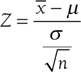
Formula reads: Z equals open parenthesis x-bar minus mu close parenthesis over open parenthesis sigma over square root of n close parenthesis.

where

is the sample mean, µ is the population mean, σ is the known population standard deviation, and n is the sample size. So, the test statistics for our example will be

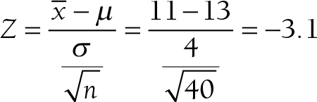
Calculation reads: Z equals open parenthesis x-bar minus mu close parenthesis over open parenthesis sigma over square root of n close parenthesis equals open parenthesis 11 minus 13 close parenthesis over open parenthesis 4 over square root of 40 close parenthesis equals negative 3.1.

based on data showing that the average number of falls for 40 participants was 11. Given the test statistic of -3.1, the p-value will be the probability to the left of -3.1 and is .001 from Figure 7-18.

Step 5: Use the p-Value to Quantify Evidence Against the Null Hypothesis

Note we had a p-value of .001 associated with the test statistic of -3.1. Conventionally, we would have compared this p-value against an arbitrarily chosen alpha value, such as .05, and concluded that the result was statistically significant. In fact, the p-value is small and would indicate that we would observe the difference as extreme as our statistic in 1 sample out of 1,000, and we will not reject the null hypothesis otherwise. However, whether the result is meaningful is a clinical/practical question, not a statistical one. In other words, it is not the p-value that determines the meaningfulness of the result; instead, it is what is clinically meaningful/effective in terms of what was measured (i.e., the number of falls in this example). So, the result of the average drop of 2 in the average number of falls from 13, with a sample mean of 11, will be meaningful, with p = .001 if it was expected to be clinically meaningful based on researchers' substantive knowledge.

As discussed earlier, it is important to support the p-value with a measure of effect size, along with a corresponding interval estimate (i.e., confidence interval) as a measure of importance. Let us discuss effect size in general, and then we will return to how we support the p-value in this example.

Effect Size ⬆ ⬇

Platts-Mills et al. (2012) found that emergency providers reported lower satisfaction with access to resident information in skilled nursing facilities (SNFs) that accept Medicaid (7.13 vs. 8.15, p< .001) versus those facilities that did not accept Medicaid. Based on these findings, should SNFs reject Medicaid funding? Can we say with any certainty that Medicaid funding is the cause of lower satisfaction? The answer to both questions is a big "No!" Statistical significance, the p-value, alone does not tell us how much of an effect was present and how important the size of the effect is in practice. Statistical significance has never answered the question of clinical meaningfulness and never will! This is, in large part, what has driven the aforementioned ASA's recommendations.

Effect size measures the strength or magnitude of an effect, difference, or relationship between variables. This computation helps us evaluate the clinical importance of study findings. Effect size may be thought of as a dose-response curve or rate. We are often exposed to this idea when evaluating how an individual patient responds to medication therapy; that is, different drug doses have varying magnitudes of effect. Aspirin prescribed at 80 mg daily has little analgesic effect, but when increased to 650 mg, aspirin has a noticeable analgesic effect. We understand that the effect of aspirin differs with the dose. We can measure similar effects of other interventions, including our fall prevention approach. An intervention with a large effect size is more likely to produce the clinical effect we seek. Therefore, effect size allows us to make a more meaningful inference from a sample to a population. Recently, many professional journals have begun to require that investigators report the effect size in their results, and the ASA recommends reporting the effect size along with a corresponding interval estimate—providing us with necessary information about the clinical significance or importance of the findings.

Types of Effect Size

There are several ways to compute an effect size, including Cohen's d, Pearson's r coefficient, ω², and others. However, we will only discuss Cohen's d and Pearson's r, the two most commonly used measures, as an introduction to effect size. In later chapters, we will discuss other types of effect sizes for different types of statistical tests.

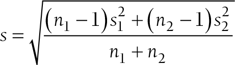
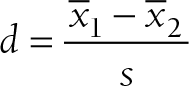
Cohen's d is simply the difference between the two population means divided by the standard deviation of the data, and it is displayed in the following formula:

Formula reads: d equals x-bar subscript 1 minus x-bar subscript 2 over s.

where s is the standard deviation of either group when the variances of the two groups are equal, or

Formula reads: s equals square root of open bracket open parenthesis n subscript 1 minus 1 close parenthesis times s subscript 1 squared plus open parenthesis n subscript 2 minus 1 close parenthesis times s subscript 2 squared all over n subscript 1 plus n subscript 2 close bracket.

when the variances of the two groups are not equal. Going back to our fall prevention example, we can use Cohen's d as an effect size for a one-sample z-test, and it will be

Calculation reads: Cohen's d equals 11 minus 13 over 4 equals negative 0.5.

Note a value of ±0.2 represents a small effect, ±0.5 represents a medium effect, and ±0.8 represents a large effect for Cohen's d (Cohen, 1988), so our result shows a medium effect, with a 95% confidence interval (9.76, 12.24), in the average number of falls. Note that the use of Cohen's definition for small, medium, and large effect sizes can be misleading. For example, Cohen's d of 0.8 indicates a large effect size, but this effect size may not mean the same in another type of effect size.

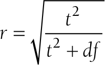
Pearson's r coefficient allows an examination of the relationship between two variables. It is the easiest coefficient to compute and interpret and can be calculated from many statistics. For example, Pearson's r coefficient as an effect size can be found by the following equation:

Formula reads: r equals square root of open parenthesis t squared over t squared plus df close parenthesis.

where t is the t-test statistic and df is the degrees of freedom. Details of these two statistics will be discussed in Chapter 11. The value varies between −1 and +1, and the effect size is small if the value varies around .1, medium if the value varies around .3, and large if the value varies around .5.

Meaning and Interpretation

Effect sizes are important because they are an objective measure of how large an effect was in a study, and they allow the nurse to consider the practical/clinical importance through the magnitude of the effect that the statistical inference cannot tell us.

As many researchers have noted the issues related to p-values, it is possible that a traditional statistically significant result may not be practically or clinically significant, and a statistically non-significant result may be practically or clinically significant (Gelman, 2015; Ioannidis, 2005, 2019; Nuzzo, 2014). For example, a study may be statistically non-significant because of a small sample size and yet demonstrate a large effect size of a newly developed intervention for preventing central line-associated bloodstream infections. Or, a study may have had a statistically significant result because of an excessively large sample size and yet have such a small effect size that application to individual patients is not possible. The practical/clinical importance of the study should be determined with careful consideration of the sample size and the purpose of the study.

Remember, we are not eliminating the use of p-values. Instead, we will use p-values to quantify evidence against the null hypothesis and support it with effect size as a measure of importance.

Statistical Power ⬆ ⬇

Statistical power is the probability of rejecting the null hypothesis when it is false or of correctly saying there is an effect when it exists. In simpler terms, statistical power helps determine the likelihood that a study will find a statistically significant result if the effect being tested is real. Remember that a Type II error (β) is the probability of not rejecting a null hypothesis when it is false or of reporting no difference in effect when there is one. Therefore, statistical power is equal to 1 - β. From this equation, we can derive that statistical power increases as the Type II error decreases, and we would want to obtain higher statistical power for the sake of our confidence in making the right conclusions.

Factors Influencing Power

Higher power is desirable in most situations, and there are several factors that can influence statistical power, including the level of significance, effect size, sample size, and the type of statistical test. The level of significance is the designated probability of making a Type I error, and you will generally obtain the greatest statistical power when you increase the level of significance because Type I errors and Type II errors are in an inverse relationship and the power is 1 - β.

Effect size is the magnitude of the relationship or difference found in a hypothesis test. When hypothesis testing produces a small p-value for a relationship or difference, it does not tell us how big the effect, relationship, or difference is—all that a small p-value says is that there is a relationship or difference. For example, the small p-value, such as .001, result we found with our two-tailed fall prevention example only tells us that the average number of falls is likely to be different from 13; it does not calculate the magnitude of the difference between the approaches. However, the effect size tells us the clinical importance of a statistical finding. In general, larger effect sizes are easier to detect, thus increasing the power of the test.

Statistical power also increases as the sample size increases. When the sample size is small, our chance of accurately representing the population is low, and the results may not be generalizable. Therefore, the probability of making the correct decision against the null hypothesis is low. The larger the sample, the more likely that the sample will represent the population and the higher the probability of making the correct decision. In other words, larger samples provide more information and reduce the variability of the estimates, making it easier to detect a true effect.

The last factor, the type of statistical test, will also influence the probability of rejecting the null hypothesis. In general, more complex statistical tests will require a larger sample size.

Types of Power Analysis

Power analyses are performed to determine the requirements to reject the null hypothesis when it should be rejected. You can conduct power analyses before or after the study is completed. A power analysis conducted before the study is completed is called an a priori power analysis, and it is a guide to determine the sample size needed to achieve a certain level of power for detecting an effect of a specific size. A post hoc power analysis is conducted after the study is completed, and it tells you what level of power the study was conducted at with the obtained sample size, along with other factors. This type of analysis can help interpret non-significant results by showing whether the study had sufficient power to detect an effect. Although a post hoc analysis is an option, investigators should always plan to conduct a priori power analysis, as it is problematic to find out that the study has low power after the study is completed. Most investigators take the minimum power of .80 as acceptable for their tests (i.e., there should be less than a 20% chance of committing a Type II error).

Meaning and Interpretations

Statistical power is the probability of rejecting a false null hypothesis or correctly saying there is an effect when it exists and is stated as a probability between 0 and 1. In other words, statistical power tells us how often we can correctly reject a null hypothesis and say there is a true effect, relationship, or difference. In interpreting the results of any study, how much power the study had in detecting an effect, if the effect exists, should be carefully considered.

Suppose an investigator wanted to determine whether ownership of hospitals (private vs. public) is related to the frequency of surgical mistakes. The investigator recruited a sample size of 104 to obtain 80% power, suggested by an a priori power analysis. If there is an actual difference in the number of surgical mistakes between public and private hospitals, it implies that this study will observe meaningful results in 80% of studies and fail to do so in the other 20% of studies.

Results from a study without enough power should be interpreted with caution, and additional studies with larger sample sizes to increase the statistical power will be required before concluding that there was an effect.

Summary ⬆ ⬇

Hypothesis testing allows researchers and clinicians to make informed decisions about the nature of research, evidence-based practice, and quality/process improvement study results by incorporating the probability of the decision being true into the decision-making process. Hypothesis testing involves five general steps: (1) stating hypotheses, (2) proposing an appropriate test, (3) checking assumptions of the chosen test, (4) computing the test statistics (finding the p-value), and (5) using the p-value to quantify evidence against the null hypothesis.

Two hypotheses, the null and alternative hypotheses, are formulated, and these are two competing statements. The hypothesis with no effects is the null hypothesis, denoted as H₀, and the hypothesis with an effect is the alternative hypothesis, denoted as H₁ or H_a.

Hypothesis testing can be either a one- or two-tailed test of inference. Two-tailed tests of inference determine only whether there is an effect, relationship, or difference, but one-tailed tests also determine the direction of the effect relationship, or difference.

Because a sample is used to make inferences about the population, there will always be a chance of making errors. In hypothesis testing, there are Type I and Type II errors. A Type I error is the probability of rejecting a true null hypothesis, and a Type II error is the probability of not rejecting a false null hypothesis. The investigator can influence error-making by selecting an acceptable sample size.

Effect size is the measure of the strength or magnitude of an effect, difference, or relationship between variables. Effect size allows us to evaluate objectively the practical or clinical worth of an intervention, the relationship between variables, or the difference between groups separately from the statistical significance.

Statistical power is the probability of rejecting a null hypothesis when it is false and equal to 1 − β. Factors such as the level of significance, effect size, sample size, and the type of statistical test affect statistical power. An a priori power analysis helps in determining sample size, given a desired power level (e.g., .80), and a post hoc power analysis helps in determining the power of specific statistical tests, given a sample size.

Critical Thinking Questions ⬆ ⬇

What is the aim of hypothesis testing?
What are the five steps of the process of statistical hypothesis testing?
What will happen to statistical power if the sample size increases?
What is the difference between statistical inference and clinical significance/ importance?
Explain the potential consequences of Type I and Type II errors in a clinical trial. Which do you think is more critical to minimize in a healthcare setting and why?
How can confidence intervals complement the results of a hypothesis test?
Explain the difference between one-tailed and two-tailed tests. When would you use each type?
Discuss the importance of effect size in the context of hypothesis testing. Why is it crucial to report effect size along with p-values?
Explain how hypothesis testing can be applied to evaluate the impact of a new nursing intervention on patient outcomes.
Why is it important to have a sufficiently large sample size when conducting hypothesis testing?

Self-Quiz ⬆ ⬇

A Type I error is made when:
1. the false null hypothesis is not rejected.
2. the true alternative hypothesis is rejected.
3. the true null hypothesis is rejected.
4. the false alternative hypothesis is not rejected.
True or False: Obtaining a statistically significant p-value (i.e., p≤ a prespecified level such as .05) is enough to conclude that there is a meaningful effect.
True or False: An investigator recently developed a new medicine and wants to test its effectiveness. The investigator collected a sample of 80 patients, divided them into control and experimental groups, and performed an experiment. The experiment showed the average difference in treating time between the control and experimental groups as above a prespecified meaningful value for a difference with the p-value of .01 and Cohen's d came out to be 0.06. The results can be concluded to be meaningful/clinically important.
What does the power of a test represent?
1. The probability of rejecting the null hypothesis when it is true
2. The probability of rejecting the null hypothesis when it is false
3. The probability of not making a Type I error
4. The probability of not making a Type II error
When is a one-tailed test appropriate?
1. When testing for any difference between groups
2. When testing for a specific direction of effect
3. When the sample size is large
4. When the significance level is .05
True or False: Effect size measures the strength of the relationship between variables.
True or False: In a two-tailed test, the rejection region is located in both tails of the distribution.
True or False: Increasing the sample size increases the power of a hypothesis test.
In hypothesis testing, what does it mean if the 95% confidence interval for a mean difference does not include zero?
1. The null hypothesis cannot be rejected.
2. The null hypothesis can be rejected.
3. The p-value is greater than .05.
4. The test has low power.
True or False: Type II error occurs when we fail to reject a true null hypothesis.

section name header

Learning Objectives ⬇

Key Concepts and Terms ⬆ ⬇

Introduction ⬆ ⬇

General Steps in Hypothesis Testing ⬆ ⬇

Hypotheses ⬆ ⬇