This chapter explains the purpose of statistical tests for determining differences between means, when to use these tests, how they are computed, and how to interpret the results. By the end of this chapter, you will be able to:
Understand approaches to difference testing to answer a proposed research question.
Distinguish an independent sample difference test from a dependent sample difference test.
Distinguish how the number of groups influences the choice of statistical test of difference.
Evaluate assumptions of difference tests.
Understand the purpose of multiple comparison testing.
Correctly report the findings of difference tests in APA style.
Understand how tests of differences are used in evidence-based practice.
Analysis of variance (ANOVA)
Bonferroni test
Dependent sample t-test
F-statistic
Independent group
Independent sample t-tests
Omega squared
One-sample t-test
One-way ANOVA
Orthogonal planned contrasts
Post hoc tests
Scheffe test
t-test
Tukey test
We use tests of mean differences, such as t-test and analysis of variance (ANOVA), to assess whether differences in health outcomes, treatment effects, or patient characteristics across groups are statistically meaningful. In health care, we are often interested in comparing one group to another or comparing treatments to determine which is more effective. Such analyses may be found in descriptive comparative and experimental investigations. For example, in a descriptive comparative investigation, we may ask how cancer incidence varies depending on sex or gender. To be more specific, we might ask, "Does the mean number of new cases of lung cancer each year differ by sex?" Descriptive comparative studies help to explain phenomena that occur naturally without the researcher influencing any variables.
We can also apply testing for substantial differences between means to experimental questions. Experimental designs are highly controlled so that the investigator can determine the effect of the independent variable on the dependent variable. We may want to know what treatment or intervention produces the best outcome, such as "On average, which wound care treatment reduces healing time the most?" In both examples, we must be able to calculate a mean value for the dependent variable to make comparisons between means; here, the average number of new lung cancer cases each year and the average time for wound healing. These tests require that dependent variables be continuous or measured at the interval or ratio level. In this chapter, we will discuss several statistical tests that compare group means of a continuous variable(s).
Case StudiesTuzon, J., & Mulkey, D. C. (2024). Implementing mobile text messaging on glycemic control in patients with diabetes mellitus. Journal of the American Association of Nurse Practitioners. https://doi.org/10.1097/JXX.0000000000001001
In 2024, Tuzon and Mulkey published their quality improvement study on using 12 weekly text messages advocating self-care measures to reduce hemoglobin A1c (HbA1c) in adults with type 2 diabetes mellitus (T2DM). Before implementing weekly text messaging, most adult patients in this rural California primary care clinic had an HbA1c of 8.5%. The American Diabetes Association (ADA) recommended an HbA1c level of less than 7%.
The investigators recruited 160 patients and implemented the American Diabetes Association's 2022 National Standard 4 of text messaging to affect change in HbA1c levels. Participants' blood samples were taken before the intervention and after 12 weekly text messages. Paired t-tests were conducted to identify if there was a change in HbA1c levels after the intervention. Their findings were displayed in a table and included mean values of HbA1c levels preintervention at 7.53% (SD = 1.72) and postintervention at 6.91% (SD = 0.89), t (159) = 11.88, p = .001.
These results were clinically significant, with a mean reduction of 0.61 (95% CI, 0.51 to 0.72) and an 8% reduction in the patient's HbA1c levels. While these results should not be generalized to other populations, this study supports the clinical value of implementing evidence-based national standards.
Tuzon and Mulkey's study is a good example of comparing differences between timed measures in a single group to determine if an intervention produces the desired effect.
Choosing the right statistical test depends upon the proposed research questions and consideration of factors such as the number of groups that will be compared. The t-test is one of the most commonly used group comparison tests and is ideal for comparing the means of two groups. When more than two groups need to be compared, researchers turn to ANOVA. A one-way ANOVA can be used to determine whether there are significant differences among the means of three or more groups.
In group comparisons, the independent variable is often called the grouping variable. In the Tuzon and Mulkey study, the independent variable was the text messaging intervention. Now, be careful, as it is easy to confuse groups with variables. For example, if the independent variable was race (one independent variable) and participants were White, Black, or Asian (three groups), we might mistakenly think there are three independent variables instead of a single grouping variableracewith the three groups. When you are designing investigations or reading reports, it is a good practice to ask yourself, "What are the independent and dependent variables in this study?"
We must also determine whether the groups are independent or dependent, which can be confusing. "Independent" refers to an investigation in which participants in one group cannot also be members of the other group. For example, if our grouping variable is age (20-30, 31-40, 41-50), then participants may be found in only one of those groups; they cannot be simultaneously 30 and 31 years old. In contrast, "dependent" refers to investigating a single group of participants when we compare the group to itself.
The t-test is the simplest statistic when comparing two means, and a one-sample t-test is the simplest t-test. A one-sample t-test compares the mean score of a sample on a continuous dependent variable to a known or hypothesized value, which is usually the population mean. This test is particularly useful in investigations that compare a sample's average outcome to a standard or established benchmark. For example, you might use a one-sample t-test to assess whether the average recovery time for a group of patients at a specific hospital differs from the national average recovery time for similar patients.
There are three assumptions for a one-sample t-test:
We must know the population mean.
The sample should be randomly selected from the population and the subjects within the sample should be independent of each other (no participant will be sampled/measured more than once).
The dependent variable should be continuous and normally distributed.
Always remember to check these assumptions before you conduct the test, as violations can limit scientific conclusions.
As with all hypotheses testing, we need to first set up the hypotheses:
H0: There is no difference between the sample mean and a known population mean.
Ha: There is a difference between the sample mean and a known population mean.
or
H0: µ = 120
Ha: µ ≠ 120.
The test statistic for a one-sample t-test can be computed by using the following formula:
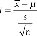
Formula reads: t equals open parenthesis x-bar minus mu close parenthesis over open parenthesis s over square root of n close parenthesis.
where

To conduct a one-sample t-test in Excel, you will open RecoveryTime.xlsx and go to Data > Data Analysis, as indicated in Figure 12-1. Note that the list does not include a one-sample t-test, but you can trick Excel and perform a one-sample t-test. First, you will type the word Average in cell B1, our label for a known population mean, and a known population mean, 120, in cells B2 and B3 (Figure 12-2). In the Data Analysis window, choose "t-Test: Two-Sample Assuming Unequal Variances" and then click "OK" (Figure 12-3). In the "t-Test: Two-Sample Assuming Unequal Variances" box, you will provide A1:A101 as Variable 1 Range and B1:B3 as Variable 2 Range with Labels selected (Figure 12-4). Clicking "OK" will then produce the output of the requested one-sample t-test; the example output is presented in Figure 12-5.
Finding Data Analysis ToolPak in Excel.
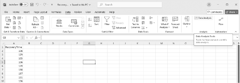
A screenshot displays an Excel worksheet with the Data tab open on the ribbon, and the Data Analysis option highlighted within the Analysis group.
Courtesy of Microsoft Excel © Microsoft 2020.
Preparing the data for Excel to compute a one-sample t-test.
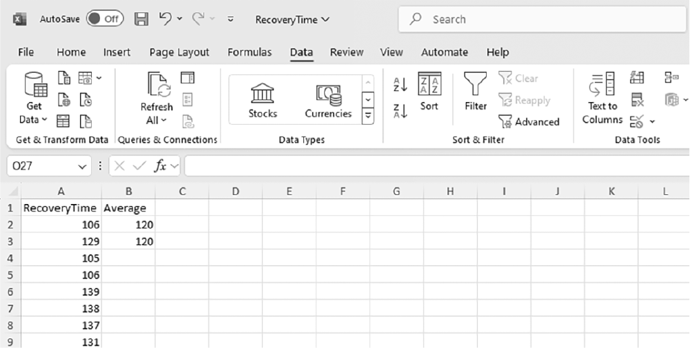
A screenshot displays an Excel spreadsheet showing a single column of numeric data with labeled column headers, ready for statistical analysis.
Courtesy of Microsoft Excel © Microsoft 2020.
Selecting a one-sample t-test within the Data Analysis ToolPak list in Excel.
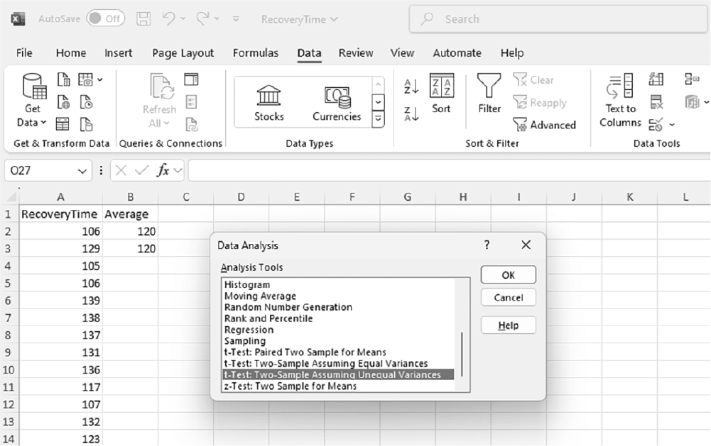
A screenshot displays the Data Analysis dialog box listing available tools, with the t-Test: One-Sample option highlighted.
Courtesy of Microsoft Excel © Microsoft 2020.
Defining data ranges and selecting options for a one-sample t-test in Excel.
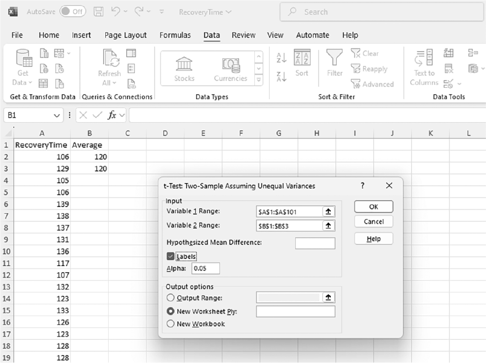
A screenshot displays the t-Test input dialog box with fields for specifying the input range, hypothesized mean, and output options.
Courtesy of Microsoft Excel © Microsoft 2020.
Example output for a one-sample t-test in Excel.
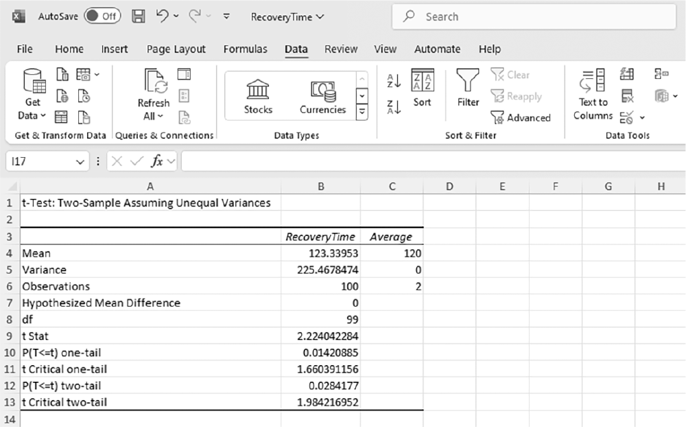
A screenshot displays a worksheet containing a results table with test statistics, degrees of freedom, p-value, and summary statistics.
Courtesy of Microsoft Excel © Microsoft 2020.
You will recognize that the average recovery time of our sample was 123.34, and the t-statistic and corresponding p-value are 2.224 and .028, respectively. A small p-value of .028 indicates that the observed difference between the sample mean and a known population mean of 3.34 units was large enough to rule out chance.
To conduct a one-sample t-test in IBM SPSS Statistics software (SPSS), you will open RecoveryTime.sav and go to Analyze > Compare means > One-sample t-test, as displayed in Figure 12-6, in this case using recovery time measurements from a sample of nursing students. In the One-Sample t-Test dialogue box, you will move RT into "Test Variable(s)" by clicking on the arrow buttons in the middle and typing in a known population mean (in this case, 120), into "Test Value" (Figure 12-7).
Selecting a one-sample t-test in SPSS.
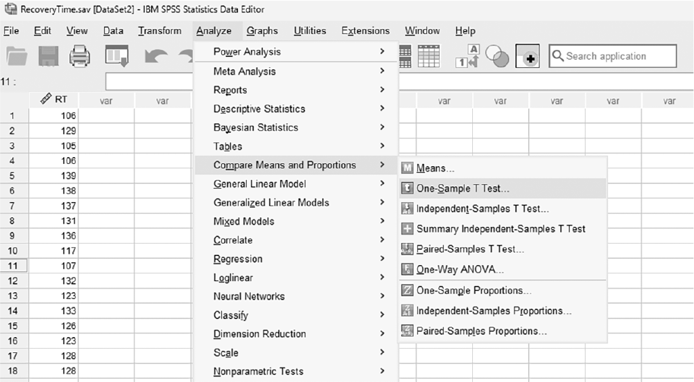
A screenshot displays a dialog box listing statistical procedures, with the One-Sample T Test option highlighted.
Reprint Courtesy of International Business Machines Corporation, © International Business Machines Corporation. "IBM SPSS Statistics software ("SPSS")". IBM®, the IBM logo, ibm.com, and SPSS are trademarks or registered trademarks of International Business Machines Corporation. Courtesy of IBM SPSS Statistics.
Defining variables in a one-sample t-test in SPSS.
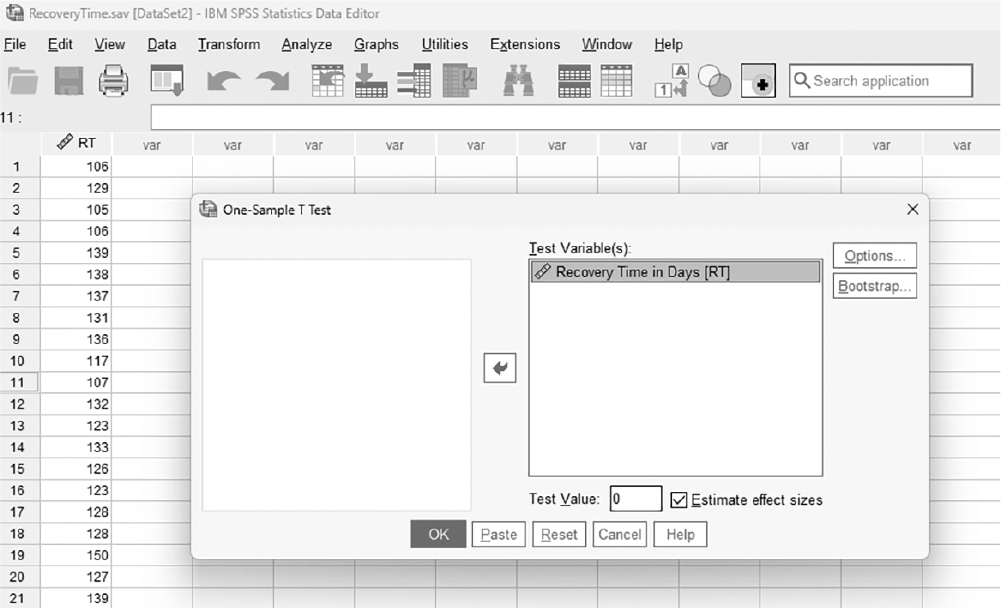
A screenshot displays a dialog box where one or more variables are selected and placed into the test variable list for analysis.
Reprint Courtesy of International Business Machines Corporation, © International Business Machines Corporation. "IBM SPSS Statistics software ("SPSS")". IBM®, the IBM logo, ibm.com, and SPSS are trademarks or registered trademarks of International Business Machines Corporation.
In the Options menu, the confidence interval can be computed based on different confidence levels, and the default is 95%. This menu also gives options for dealing with missing values. The default is to "exclude cases by analysis," which excludes cases if they have missing values on variables in the current analysis. The other option is to "exclude cases listwise"; this option deletes cases with missing values on any variables, whether in the current or prior analysis. If cases have even one missing value on a single variable, they will be excluded from the entire analysis, and the analysis is run only on those with complete values. Clicking "OK" will produce the requested t-test analysis output. The example output is presented in Table 12-1.
One-Sample Statistics | |||||||
|---|---|---|---|---|---|---|---|
N | Mean | Std. Deviation | Std. Error Mean | ||||
Recovery Time in Days | 100 | 123.34 | 15.016 | 1.502 | |||
One-Sample Test Test Value= 0 | |||||||
Significance | 95% Confidence Interval of the Difference | ||||||
t | df | One-Sided p | Two-Sided p | Mean Difference | Lower | Upper | |
Recovery Time in Days | 82.141 | 99 | <.001 | <.001 | 123.340 | 120.36 | 126.32 |
One-Sample Effect Sizes | |||||||
95% Confidence Interval | |||||||
Standardizera | Point Estimate | Lower | Upper | ||||
Recovery Time in Days | Cohen’s d | 15.016 | 8.214 | 7.054 | 9.372 | ||
Hedges’ correction | 15.131 | 8.152 | 7.000 | 9.300 | |||
a. The denominator used in estimating the effect sizes. Cohen’s d uses the sample standard deviation. Hedges’ correction uses the sample standard deviation, plus a correction factor. | |||||||
Note that the average recovery time was 123.34, the same as that in Excel, with the t-statistic and corresponding p-value of 2.224 and .028, respectively. Again, a small p-value of .028 indicates that the difference of 3.34 units in recovery time between the sample and the population was large enough to rule out chance.
When reporting one-sample t-test results, you should report the size of the t-statistic, the associated p-value, and means and standard error so that readers will know how the sample statistic is different from the known population parameter. Cohen's d, a type of effect size as discussed in Chapter 7, should also be computed and reported. Results of the t-test for our example for IQ variable could be reported in this way:
Patients at ABC hospital had higher average recovery time (M = 123.34, SE = 1.50) than the national average recovery time for similar patients, t (99) = 2.22, p = .028, d = .22, 95% CI [0.36, 6.32].
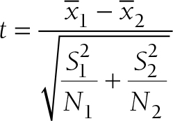
Independent sample t-tests are used when two independent groups are compared on their means. By "independent," we mean that the subjects in one group cannot also be members of the other group. The t-statistic is computed by dividing the difference between means by an estimate of the standard error of the difference between those two independent sample means. A large deviation between means suggests that the samples from the population differ a lot, and a small deviation between means suggests that samples from the population are more similar.
In t-tests, the standard error is used to gauge the variability between sample means. When the standard error is large, we will observe large differences in sample means and small differences in sample means when the standard error is small. For example, in experimental studies, where we often compare treatments or interventions, we reject the null hypothesis when the sample means between the treatment and control groups are substantially different. Otherwise, the difference between sample means occurs by chance only.
The following parametric assumptions should be met before the independent samples t-test is computed.
The sampling distribution should be normal (i.e., the dependent variable should be normally distributed).
The data should be measured at the interval level, at least (i.e., continuous measurement).
Measurements should be independent (i.e., subjects in these two groups should not overlap).
Variances in the compared groups should be about the same.
Please refer to Chapter 8 for the details about how to check these assumptions.
First, we need to set up hypotheses:
H0: There is no difference between group 1 mean and group 2 mean.
Ha: There is a difference between group 1 mean and group 2 mean.
or
H0: µ1= µ2
Ha: µ1≠µ2.
The test statistic for independent samples t-test can be found by using one of the following formulas:

Formula reads: t equals open parenthesis x-bar subscript 1 minus x-bar subscript 1 close parenthesis over square root of open bracket open parenthesis S subscript 1 squared over N subscript 1 close parenthesis plus open parenthesis S subscript 2 squared over N subscript 2 close parenthesis close bracket.
when sample sizes are equal; or

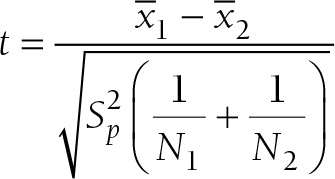
Formula reads: t equals (x-bar subscript 1 minus x-bar subscript 1) over square root of [S subscript p squared times (1 over N subscript 1 plus 1 over N subscript 2)].
when sample sizes are not equal
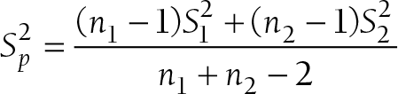
where

Formula reads: S subscript p squared equals open bracket open parenthesis n subscript 1 minus 1 close parenthesis times S subscript 1 squared plus open parenthesis n subscript 2 minus 1 close parenthesis times S subscript 2 squared close bracket over open bracket n subscript 1 plus n subscript 2 minus 2 close bracket.
If the observed difference between the two means is substantial and the associated p-value is small, we may rule out chance as influencing the difference. When the observed difference is not substantial, and the associated p-value is large, that indicates that chance is likely influencing the outcome. As discussed earlier, it is important to support the p-value with a measure of effect size and a corresponding interval estimate (i.e., confidence interval) as a measure of importance.
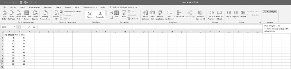
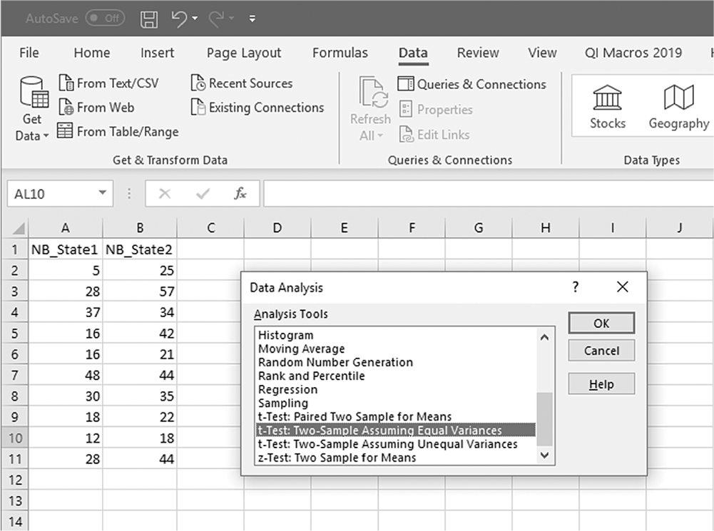
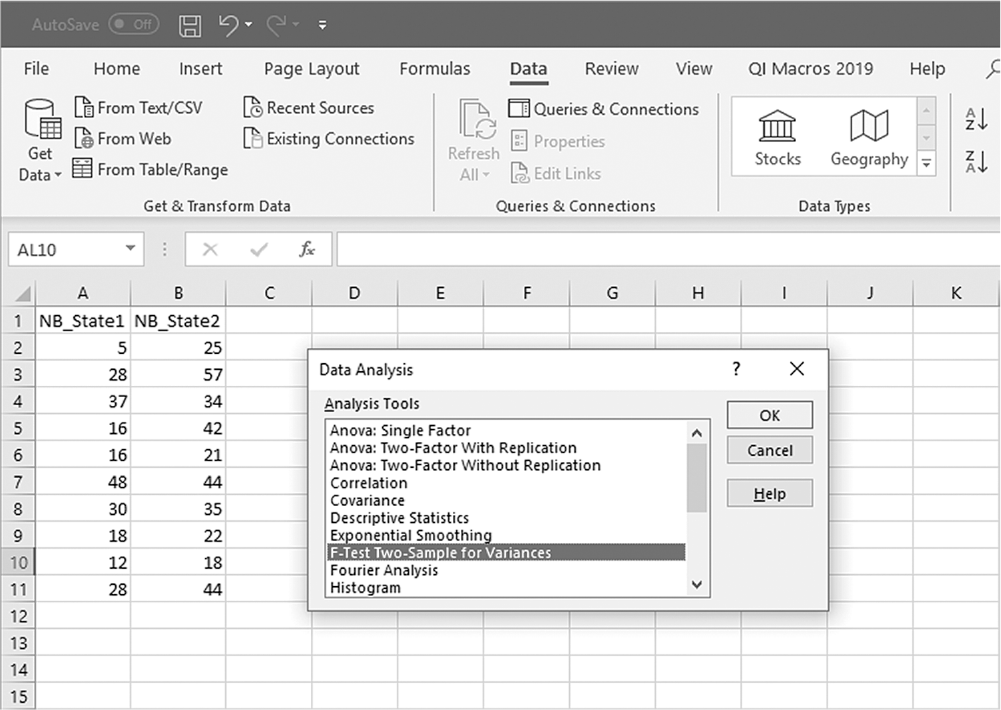
To conduct an independent samples t-test in Excel, you will open NumberBed.xlsx (the data presented in Figure 12-8 are the number of beds in nursing homes in the states of Illinois and Ohio) and go to Data > Data Analysis, as displayed in the figure. In the Data Analysis window, you will note that there are "t-Test: Two-Sample Assuming Equal Variances" and "t-Test: Two-Sample Assuming Unequal Variances" on the list (Figure 12-9). So, the first thing that you will need to do is to figure out whether the variances of the two groups are equal and choose "F-Test Two-Sample for Variances," as displayed in Figure 12-10. This test will check the following hypotheses:
Finding Data Analysis ToolPak in Excel.
An Excel screenshot shows the Data Analysis ToolPak add-in, in the Analysis group under Data menu.
Courtesy of Microsoft Excel © Microsoft 2020.
Two different independent samples t-tests within the Data Analysis ToolPak in Excel.
An Excel screenshot shows selection of the option, t-Test: Two-Sample Assuming Unequal Variances, within the Data Analysis ToolPak. The worksheet shows two columns, with headings, N B_State 1 and N B_State 2, containing numerical data.
Courtesy of Microsoft Excel © Microsoft 2020.
Selecting "F-Test Two-Sample for Variances" in Excel.
An Excel screenshot shows selection of the option, F-Test Two-Sample for Variances, within the Data Analysis ToolPak. The worksheet shows two columns, with headings, N B_State 1 and N B_State 2, containing numerical data.
Courtesy of Microsoft Excel © Microsoft 2020.
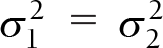
H0: Variances of the two groups are equal.
HA: Variances of the two groups are not equal.
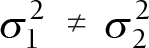
or
H0:

Ha :

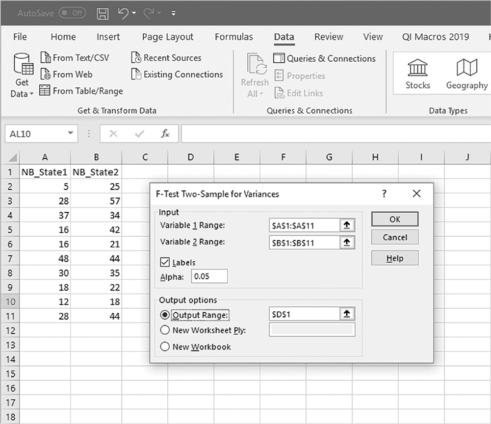
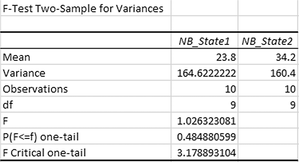
The assumption of equal variance is said to be violated when the p-value is too small to rule out chance, and the assumption is said to be not violated otherwise. In the "F-Test Two-Sample for Variances" dialogue box, you will provide A1:A11 as Variable 1 Range, B1:B11 as Variable 2 Range, and D1 as Output Range with Labels selected (Figure 12-11). Clicking "OK" will then produce the requested regression analysis output; the example output is demonstrated in Figure 12-12.
Defining data ranges and selecting options for "F-Test Two-Sample for Variances" in Excel.
An Excel screenshot shows a dialog box with the inputting of data ranges and selecting output options for a one-sample F-test. The worksheet lists N B_State 1 and N B_State 2, with numerical data.
The dialog box, with heading F-Test Two-Sample for Variances, has two textboxes. The first textbox with heading, Input, consists of two drop-down lists, Variable 1 range and Variable 2 range; there is an option, Labels, which is checked. The second textbox with heading, Output options, consists of a drop-down list, output range, which is checked and value D 1 entered; new worksheet ply; and new worksheet. The buttons, O k, Cancel, and Help, are on the right of the dialog box.
Courtesy of Microsoft Excel © Microsoft 2020.
Example output for "F-Test Two-Sample for Variances" in Excel.
An Excel screenshot displays the output for a one-sample F-test.
The heading of a table reads, F-Test: Two-Sample for Variances. The output has three columns, no data, N B_State 1, and N B_State 2. The row entries are as follows. Row 1: Mean, 23.8, 34.2. Row 2: Variance: 164.6222222, 160.4. Row 3: Observations, 10, 10. Row 4: d f, 9, 9. Row 5: F, 1.0263323081, no data. Row 6: P of F less than or equal to fone-tail, 0.0484880599, no data. Row 8: F critical one-tail, 3.178893104, no data.
Courtesy of Microsoft Excel © Microsoft 2020.
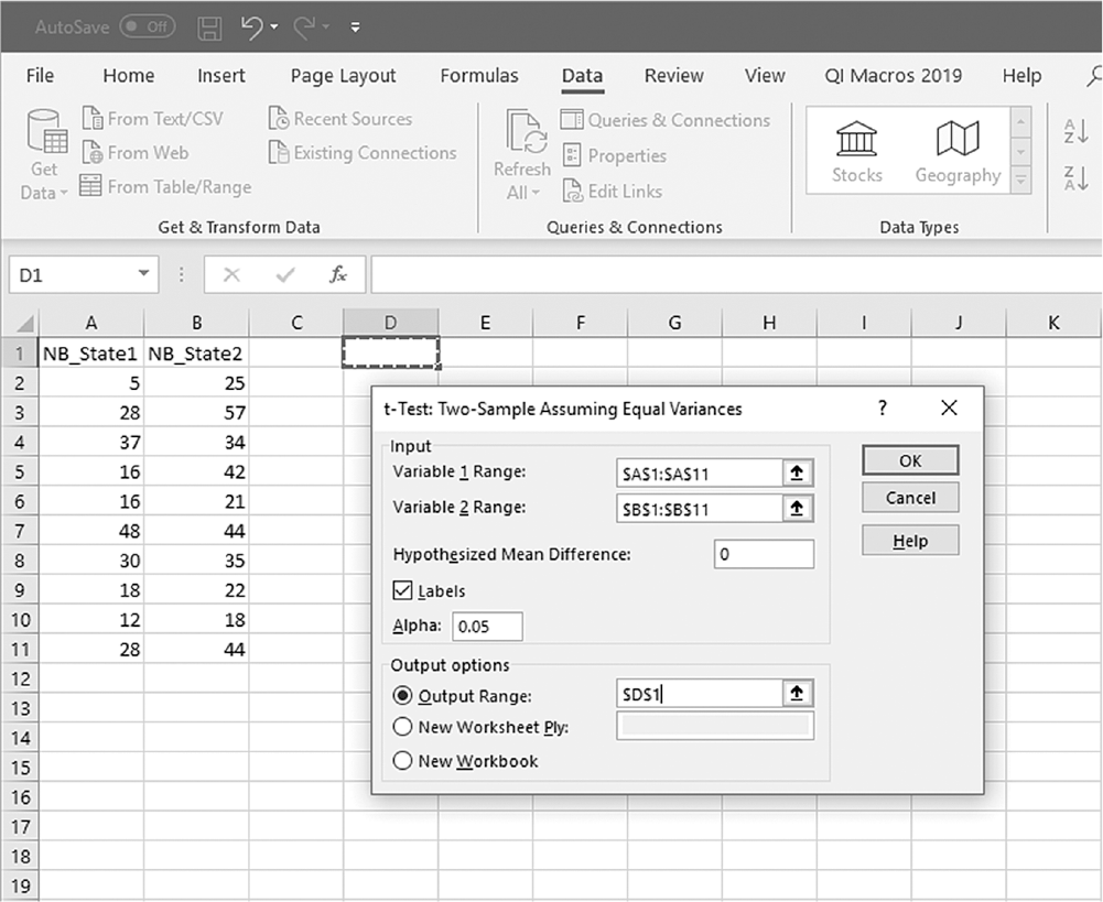
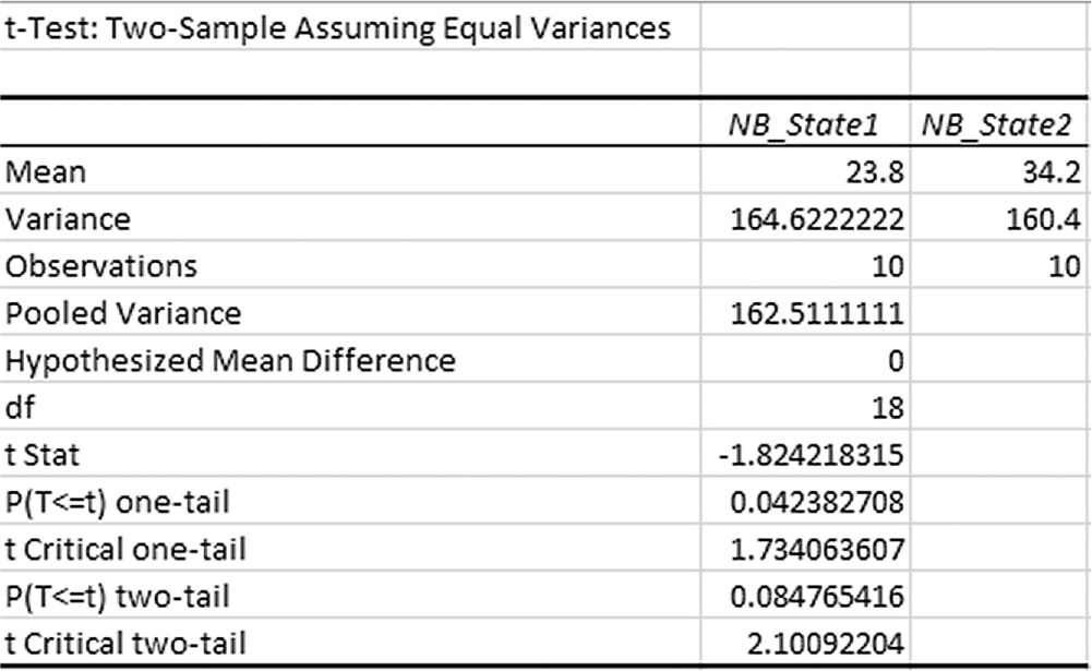
Note that the associated p-value with the F statistic is 0.485, so the observed difference between the two variances is not large enough to rule out chance. Therefore, we will select "t-Test: Two-Sample Assuming Equal Variances" in Figure 12-9 and use it to test for the difference between the two average number of beds. In the "t-Test: Two-Sample Assuming Equal Variances" dialogue box, you will provide A1:A11 as Variable 1 Range, B1:B11 as Variable 2 Range, "0" for Hypothesized Mean Difference, and D1 as output range with Labels selected (Figure 12-13). Clicking "OK" will then produce the output of the requested regression analysis, and the example output is presented in Figure 12-14.
Defining data ranges and selecting options for "t-Test: Two-Sample Assuming Equal Variances" in Excel.
An Excel screenshot shows a dialog box with the inputting of data ranges and selecting output options for a two-sample t-test. The worksheet lists N B_State 1 and N B_State 2, with numerical data.
The dialog box, with heading t-Test: Two-Sample Assuming Equal Variances, has two textboxes. The first textbox with heading, Input, consists of two drop-down lists, Variable 1 range and Variable 2 range; there is an option, Labels, which is checked. The entry field, hypothesized mean difference has the value 0 entered, and Alpha has 0.05 entered in it. The second textbox with heading, Output options, consists of a drop-down list, output range which is checked; new worksheet ply; and new worksheet. The buttons, O k, Cancel, and Help, are on the right of the dialog box.
Courtesy of Microsoft Excel © Microsoft 2020.
Example output for "t-Test: Two-Sample Assuming Equal Variances" in Excel.
An Excel screenshot displays the output for a two-sample t-test.
The heading of a table reads, t-Test: Two-Sample assuming Equal Variances. The output has three columns, no data, N B_State 1, and N B_State 2. The row entries are as follows. Row 1: Mean, 23.8, 34.2. Row 2: Variance: 164.6222222, 160.4. Row 3: Observations, 10, 10. Row 4: Pooled variance, 162.5111111, no data. Row 5: Hypothesized mean difference, 0, no data. Row 6: d f, 18, no data. Row 7: t Stat, minus 1.824218315, no data. Row 8: P of T less than or equal to tone-tail, 0.042382708, no data. Row 9: t critical one-tail, 1.734063607, no data. Row 9: P of T less than or equal to ttwo-tail, 0.084765416, no data. Row 9: t critical two-tail, 2.10092204, no data.
Courtesy of Microsoft Excel © Microsoft 2020.
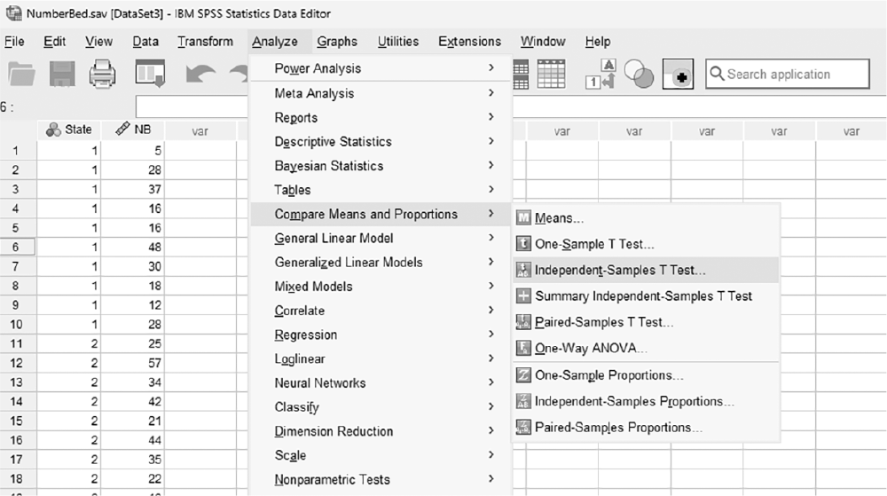
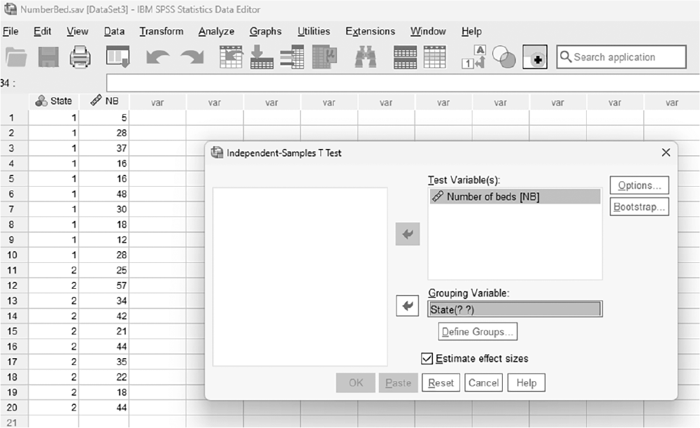
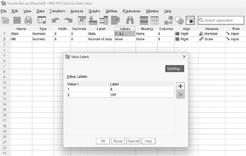
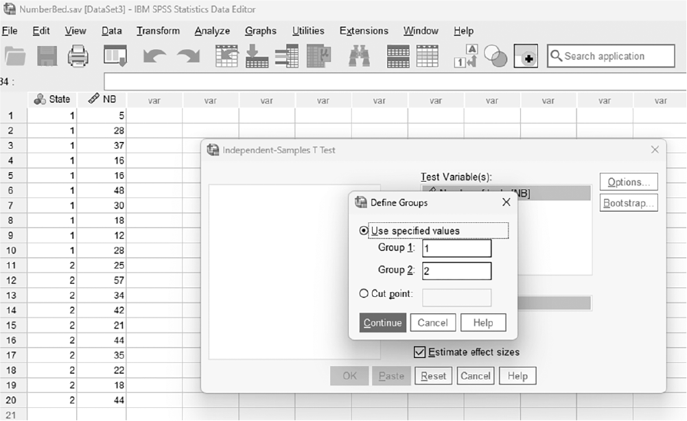
To conduct an independent samples t-test in SPSS, you will open NumberBed.sav and go to Analyze > Compare means > Independent samples t-test, as displayed in Figure 12-15. In the Independent Samples t-Test dialogue box, you will move a dependent variable, "NB," into "Test Variable(s)" and the independent variable, "State," into "Grouping Variable" by clicking the corresponding arrow buttons in the middle, as displayed in Figure 12-16. You will notice that the "OK" button is inactive because we have not defined our two groups. As you notice in Figure 12-17, we have defined the coding of 1 for Illinois and 2 for Ohio. Click on the "Define Groups" button and assign 1 for Group 1 (Illinois) and 2 for Group 2 (Ohio) (Figure 12-18). Clicking "Continue" and then "OK" will produce the output of the requested analysis. The example output is displayed in Table 12-2.
Selecting an independent samples t-test in SPSS.
A screenshot displays a dialog box listing statistical tests, with the Independent-Samples T Test option highlighted for selection.
Reprint Courtesy of International Business Machines Corporation, © International Business Machines Corporation. "IBM SPSS Statistics software ("SPSS")". IBM®, the IBM logo, ibm.com, and SPSS are trademarks or registered trademarks of International Business Machines Corporation.
Defining variables in an independent samples t-test in SPSS.
A screenshot displays a dialog box where one variable is placed in the test variable field and another variable is placed in the grouping variable field.
Reprint Courtesy of International Business Machines Corporation, © International Business Machines Corporation. "IBM SPSS Statistics software ("SPSS")". IBM®, the IBM logo, ibm.com, and SPSS are trademarks or registered trademarks of International Business Machines Corporation.
Coding scheme for "State" variable.
A screenshot displays a data view table showing a column labeled State with numeric codes assigned to represent different categories.
Reprint Courtesy of International Business Machines Corporation, © International Business Machines Corporation. "IBM SPSS Statistics software ("SPSS")". IBM®, the IBM logo, ibm.com, and SPSS are trademarks or registered trademarks of International Business Machines Corporation.
Defining groups in an independent samples t-test in SPSS.
A screenshot displays a dialog box with two input boxes labeled for group identifiers, showing numeric values entered to define comparison groups.
Reprint Courtesy of International Business Machines Corporation, © International Business Machines Corporation. "IBM SPSS Statistics software ("SPSS")". IBM®, the IBM logo, ibm.com, and SPSS are trademarks or registered trademarks of International Business Machines Corporation.
Group Statistics | |||||||||||
|---|---|---|---|---|---|---|---|---|---|---|---|
State | N | Mean | Std. Deviation | Std. Error Mean | |||||||
Number of beds | IL | 10 | 23.80 | 12.831 | 4.057 | ||||||
OH | 10 | 34.20 | 12.665 | 4.005 | |||||||
Independent Samples Test | |||||||||||
t-Test for Equality of Means | |||||||||||
Levene’s Test for Equality of Variances | Significance | 95% Confidence Interval of the Difference | |||||||||
F | Sig. | t | df | One-Sided p | Two-Sided p | Mean Difference | Std. Error Difference | Lower | Upper | ||
Number of beds | Equal variances assumed | 0.004 | 0.947 | μ1.824 | 18 | 0.042 | 0.085 | -10.400 | 5.701 | -22.378 | 1.578 |
Equal variances not assumed | μ1.824 | 17.997 | 0.042 | 0.085 | -10.400 | 5.701 | -22.378 | 1.578 | |||
Independent Samples Effect Sizes | |||||||||||
95% Confidence Interval | |||||||||||
Standardizera | Point Estimate | Lower | Upper | ||||||||
Number of beds | Cohen’s d | 12.748 | μ0.816 | μ1.721 | 0.110 | ||||||
Hedges’ correction | 13.312 | μ0.781 | μ1.648 | 0.105 | |||||||
Glass’s delta | 12.665 | μ0.821 | μ1.755 | 0.151 | |||||||
a. The denominator used in estimating the effect sizes. Cohen’s d uses the pooled standard deviation. Hedges’ correction uses the pooled standard deviation, plus a correction factor. Glass’s delta uses the sample standard deviation of the control group. | |||||||||||
Notice that the average number of nursing home beds per nursing home in Illinois is 23.8, and in Ohio, the average is 34.2. On average, we notice that there is about a 10-bed difference between the two states; the question is whether this difference of 10 beds is substantial. Recall that one of the assumptions was that the variability of the two groups is about the same. Independent samples t-test outputs in SPSS include the results of Levene's test, which checks this assumption.
The assumption of equal variance is said to be violated when the p-value is too small to rule out chance, and the assumption is said not to be violated otherwise. You should interpret the results of an independent samples t-test according to this result. If the equal variance assumption is met, you should interpret the first row of the output, "Equal variances assumed," and the second row of the output, "Equal variances not assumed," if the equal variance assumption is unmet. In our example, the assumption of equal variances is not violated, so we will interpret the "Equal variances assumed" row of the output. The computed t-statistic and corresponding p-value are -1.824 and .085, respectively. Because the p-value is large, the null hypothesis is not rejected, and it is determined that the average number of beds in Illinois and Ohio nursing homes is said to be roughly the same.
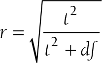
When reporting independent samples t-test results, you should report the size of the t-statistic and associated p-value and also report means and standard error so that the readers will know how the two sample means differ. Another type of effect size, r, as discussed in Chapter 7, can be computed with the following equation:

Formula reads: t equals square root of t squared over t squared plus df.
and reported for the independent sample t-test. The following is a sample report for this example:
On average, the number of beds in Illinois nursing homes (M = 23.8, SE = 4.06) was not different from the number of beds in Ohio nursing homes (M = 34.2, SE = 4.01), t(18) = -1.83, p = .085, r = .40, 95% CI [-22.38, 1.58].
We use the dependent sample t-test when the measurements of a given dependent variable are paired. By dependent samples, we mean that we are dealing with a single group of participants; therefore, their responses to one set of measurements are related to another. There are two ways that measurements can be paired. First, one sample can be measured twice, such as when a group of patients' systolic blood pressure (SBP) was measured before and after they received an antihypertensive drug. Second, two different data sets can be paired, such as in the Turzon case study, when a group of participants had their HgA1c measured at two different times. The statistic is computed in the same way as in the independent samples t-test, in that the difference between the means is divided by some form of the standard error. Measurements will differ a lot if there is a large deviation between means, and measurements will not differ much if there is a small deviation between means. The same rationale discussed previously for the independent samples t-test still applies to the dependent samples t-test.
As measurements will not be independent, we cannot assume that the last two assumptions of the independent t-test, which are the assumptions of equal variance and independent measurements, are valid. However, the normality of sampling distribution and data being measured at the interval level still apply.
One thing to note about the two assumptions for a dependent samples t-test is that what has to be measured at least at the interval level and to be normally distributed are not the measurements themselves. It is, in fact, the difference between the two sets of measurements that must be measured at the interval level and normally distributed. For example, we need to check the level of measurement and normality of the difference between systolic blood pressure measurements before and after receiving an antihypertensive drug, not the before and after measurements themselves. Therefore, the first task is to calculate the difference between the measurements for each case in the data set, and then you should examine the level of measurements and the normality of it.
First, we need to set up hypotheses:
H0: There is no difference between before measurements and after measurements.
Ha: There is a difference between before measurements and after measurements.
or
H0: µB= µA
Ha: µB≠µA.
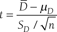
The test statistic for dependent samples t-test can be found by the following equation:

where

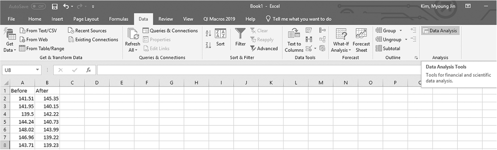
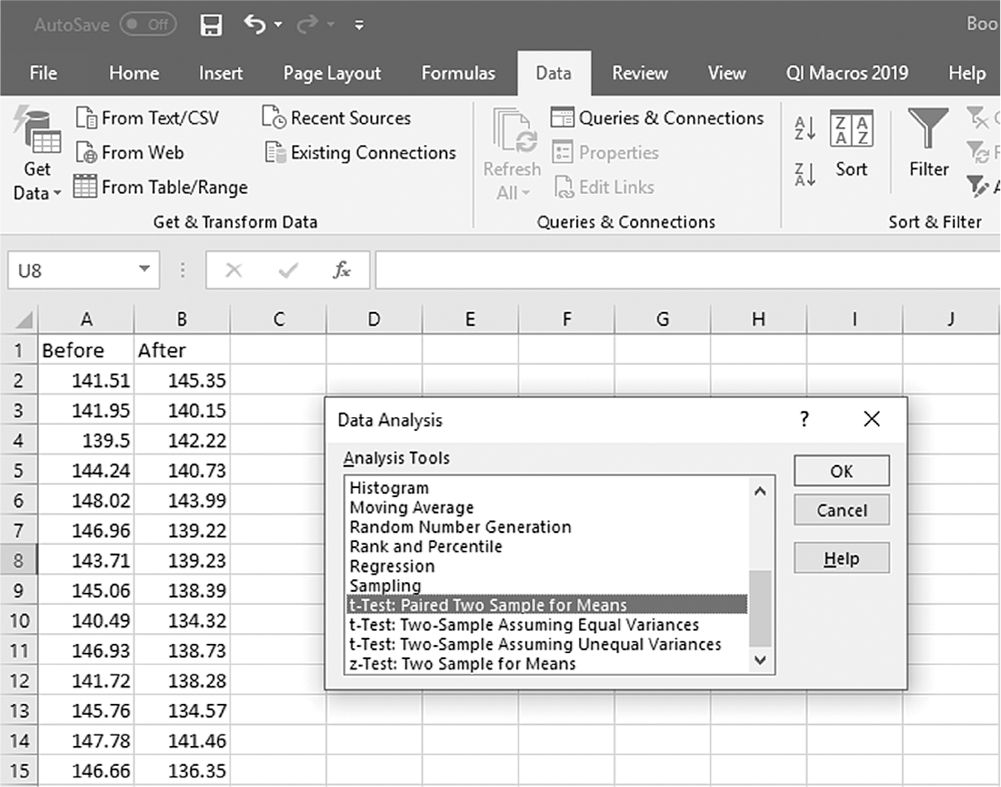
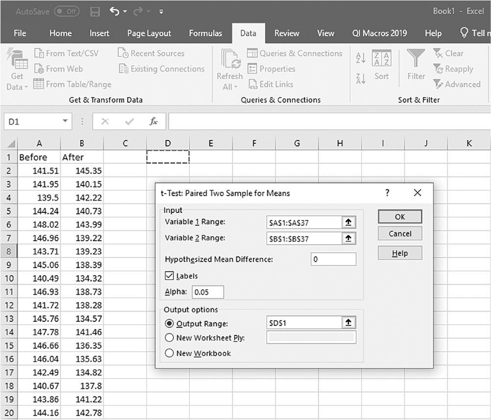
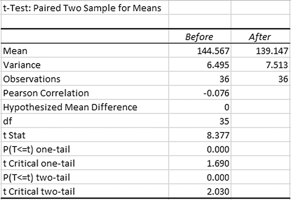
To conduct a dependent samples t-test in Excel, you will open SodiumContent.xlsx and go to Data > Data Analysis, as displayed in Figure 12-19. In the Data Analysis window, choose "t-Test: Paired Two Sample for Means" in the list and then click "OK" (Figure 12-20). In the Linear "t-Test: Paired Two Sample for Means" dialogue box, you will provide A1:A11 as Variable 1 Range, B1:B11 as Variable 2 Range, "0" for Hypothesized Mean Difference, and D1 as output range with Labels selected (Figure 12-21). Clicking "OK" will then produce the output of requested regression analysis, and the example output is displayed in Figure 12-22.
Finding Data Analysis ToolPak in Excel.
An Excel screenshot shows the Data Analysis ToolPak add-in, in the Analysis group under Data menu.
Courtesy of Microsoft Excel © Microsoft 2020.
Selecting "t-Test: Paired Two Sample for Means" in Excel.
An Excel screenshot shows selection of the option, t-Test: Paired Two Sample for Means, within the Data Analysis ToolPak. The worksheet shows two columns, with headings, Before and After, containing numerical data.
Courtesy of Microsoft Excel © Microsoft 2020.
Defining data ranges and selecting options for "t-Test: Paired Two Sample for Means" in Excel.
An Excel screenshot shows a dialog box with the inputting of data ranges and selecting output options for a two-sample t-test. The worksheet lists Before and After, with numerical data.
The dialog box, with heading t-Test: Paired Two Sample for Means, has two textboxes. The first textbox with heading, Input, consists of two drop-down lists, Variable 1 range and Variable 2 range; there is an option, Labels, which is checked. The entry field, hypothesized mean difference has the value 0 entered, and Alpha has 0.05 entered in it. The second textbox with heading, Output options, consists of a drop-down list, output range which is checked and the cell D 1 entered; new worksheet ply; and new worksheet. The buttons, O k, Cancel, and Help, are on the right of the dialog box.
Courtesy of Microsoft Excel © Microsoft 2020.
Example output for "t-Test: Paired Two Sample for Means" in Excel.
An Excel screenshot displays the output of requested regression analysis.
The heading of a table reads, t-Test: Paired Two Sample Means. The output has three columns, no data, Before, and After. The row entries are as follows. Row 1: Mean, 144.567, 139.147. Row 2: Variance: 6.495, 7.513. Row 3: Observations, 36, 36. Row 4: Pearson correlation, minus 0.076, no data. Row 5: Hypothesized mean difference, 0, no data. Row 6: d f, 35, no data. Row 7: t Stat, 8.377, no data. Row 8: P of T less than or equal to tone-tail, 0.000, no data. Row 9: t critical one-tail, 1.690, no data. Row 9: P of T less than or equal to ttwo-tail, 0.000, no data. Row 9: t critical two-tail, 2.030, no data.
Courtesy of Microsoft Excel © Microsoft 2020.
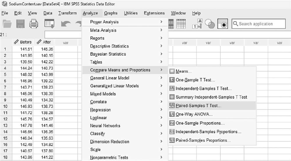
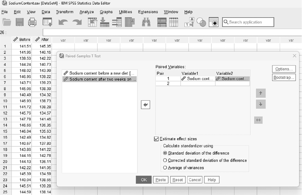
To conduct a dependent samples t-test in SPSS, you will open SodiumContent.sav and go to Analyze > Compare means > Paired samples t-test, as displayed in Figure 12-23. The data presented in this figure are the sodium content levels in a sample of patients both before and after a new diet. In the Paired Samples t-Test dialogue box, then you will move the variables to be paired into "Paired Variables" in order by clicking the corresponding arrow buttons in the middle, as displayed in Figure 12-24. Clicking "OK" will then produce the output of the requested analysis. An example output is presented in Table 12-3.
Selecting a dependent samples t-test in SPSS.
A screenshot displays a dialog box listing statistical tests, with the Paired-Samples T Test option highlighted for selection.
Reprint Courtesy of International Business Machines Corporation, © International Business Machines Corporation. "IBM SPSS Statistics software ("SPSS")". IBM®, the IBM logo, ibm.com, and SPSS are trademarks or registered trademarks of International Business Machines Corporation.
Defining variables in a dependent samples t-test in SPSS.
A screenshot displays a dialog box where two variables are paired and placed into fields labeled for the first and second measurements for analysis.
Reprint Courtesy of International Business Machines Corporation, © International Business Machines Corporation. "IBM SPSS Statistics software ("SPSS")". IBM®, the IBM logo, ibm.com, and SPSS are trademarks or registered trademarks of International Business Machines Corporation.
Paired Samples Statistics | ||||||||||
|---|---|---|---|---|---|---|---|---|---|---|
Mean | N | Std. Deviation | Std. Error Mean | |||||||
Pair 1 | Sodium content before a new diet | 144.5666 | 36 | 2.54909 | 0.42485 | |||||
Sodium content after 2 weeks on a new diet | 139.1459 | 36 | 2.74068 | 0.45678 | ||||||
Paired Samples Correlations | ||||||||||
Significance | ||||||||||
N | Correlation | One-Sided p | Two-Sided p | |||||||
Pair 1 | Sodium content before a new diet and sodium content after 2 weeks on a new diet | 36 | μ0.076 | 0.329 | 0.658 | |||||
Paired Samples Test | ||||||||||
|---|---|---|---|---|---|---|---|---|---|---|
Paired Differences | ||||||||||
95% Confidence Interval of the Difference | Significance | |||||||||
Mean | Std. Deviation | Std. Error Mean | Lower | Upper | t | df | One-Sided p | Two-Sided p | ||
Pair 1 | Sodium content before a new diet and sodium content after 2 weeks on a new diet | 5.42061 | 3.88285 | 0.64714 | 4.10684 | 6.73438 | 8.376 | 35 | <.001 | <.001 |
Paired Samples Effect Sizes | ||||||||||
95% Confidence Interval | ||||||||||
Standardizera | Point Estimate | Lower | Upper | |||||||
Pair 1 | Sodium content before a new diet and sodium content after 2 weeks on a new diet | Cohen’s d | 3.88285 | 1. 396 | 0.93 | 1.852 | ||||
Hedges’ correction | 3.96861 | 1.366 | 0.909 | 1.812 | ||||||
a. The denominator used in estimating the effect sizes. Cohen’s d uses the sample standard deviation of the mean difference. Hedges’ correction uses the sample standard deviation of the mean difference, plus a correction factor. | ||||||||||
Observe that the average sodium content level before the new diet is 144.6 units, and the average sodium content level after a new diet is 139.1 units. We notice a difference of 5.4 units in sodium content level between the before and after measurements. The question is whether this difference of 5.4 units of sodium is meaningful. The second section in Table 12-3 shows that the measurements are not substantially correlated, with a correlation coefficient of -.08 and its associated p-value of .658. The computed t-statistic and corresponding p-value are 8.376 and .000, respectively. Because the p-value of .000 is extremely small, we reject the null hypothesis, having determined that the average sodium content level before the new diet is substantially higher than the one measured after the new diet.
When reporting dependent samples t-test results, you should report the size of the t-statistic, associated p-value, and the means and standard error so that readers will know how the before and after sample means differ. Like the independent samples t-test, r can be computed and reported for the dependent sample t-test. The following is a sample report from our example:
On average, the sodium content level after the new diet (M = 144.6, SE = 0.42) was substantially lower than that before the new diet (M = 139.1, SE = 0.46), t (35) = 8.38, p = .000, r = .82, 95% CI [4.11, 6.73].
The independent t-test allows us to compare the means of two independent groups and decide whether these are different. But what if we have more than two groups to compare? For example, a nurse investigator is interested in testing the effectiveness of a newly developed diet using three groups: a placebo group, an existing diet group, and a new diet group. Because the independent t-test is only designed to test two group means, the simultaneous comparison of these three groups is impossible. You may think it is possible to conduct three independent samples t-tests by comparing the following pairs: placebo-existing diet, placebo-new diet, and existing diet-new diet. However, there is an increased risk of Type I error if we conduct multiple tests this way, and this increased risk gets worse as the number of tests increases (i.e., the actual risk of Type I error will increase as the number of tests increases). This will be true for any set of statistical tests.
For any given set of statistical tests, the inflated Type I error will be:
αinflated = 1 - (1 - αprespecified)n
where αinflated is the inflated Type I error after conducting multiple tests, αprespecified is the prespecified/desired Type I error, and n is the One-Way Analysis of Variance231number of tests. As you notice, the risk of Type I error will be inflated as more tests are conducted. For example, if you conduct three tests, each at a Type I error of .05, the Type I error is inflated to
αinflated = 1 - (1 - .05)3 = .1426
and running five tests will inflate the Type I error to
αinflated = 1 - (1 - .05)5 = .2262
So, what do .1426 and .2262 mean? They mean that you have a higher probability of committing a Type I error by conducting multiple tests (i.e., you will be more likely to falsely reject the true null hypothesis). Therefore, you should control for an inflated Type I error somehow so that you will not incorrectly reject the true null hypothesis more frequently than you desired.
A better statistical test to identify three or more group differences is an analysis of variance (ANOVA), which compares all groups simultaneously and captures the overall differences across groups. However, ANOVA only indicates that there exists a group difference; it does not depict specifically which groups differ. We offer an example of this in the next section.
All assumptions of an independent samples t-test also apply to one-way ANOVA, as it is a natural extension of an independent samples t-test. These parametric assumptions are as follows:
The sampling distribution should be normal (i.e., the dependent variable should be normally distributed).
The dependent variable data should be measured at least on an interval level (i.e., continuous measurement).
Variances in the groups in the comparison should be about the same.
The measurements should be independent (i.e., subjects in the groups should not overlap).
Please refer again to Chapter 9 for details about how to check these assumptions.
First, we need to set up hypotheses:
H0: There is no difference among group means.
Ha: At least two group means differ.
or
H0: µ1= µ2= µ3
Ha: µj≠µkfor some j and k
Again, the alternative hypothesis cannot be written as
Ha: µj≠µkfor all j and k
because we do not know if all groups differ or if just two or three groups differ. The test statistic for one-way analysis of variance can be found by the following equation:

Formula reads: F equals Differences between groups over Differences within groups.
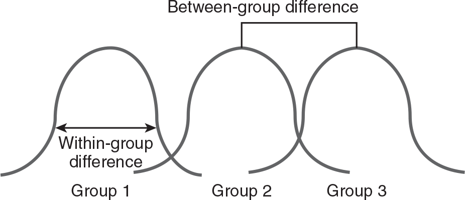
where both differences are presented in Figure 12-25. A small p-value, such as .000, would lead us to reject the null hypothesis, indicating that the groups differ because it would indicate that we would observe a difference as extreme as our statistic in almost zero samples out of 1,000, and we will not reject the null hypothesis otherwise. From the figure, it is clear that the differences between groups will be more likely to be present as the difference between groups gets larger (i.e., the statistic will likely fall in the rejection region as it gets larger).
Visual representation of between- and within-group differences.
An illustration depicts between-group differences and within-group differences, where each group is represented as a bell-shaped curve.
Group 1 at the left overlaps with Group 2 curve at the center and Group 2 overlaps with Group 3 on the right. The amount of overlap between Group 1 and Group 2 is less compared to that between Group 2 and Group 3. Within-group difference is indicated by a double-headed horizontal arrow in Group 1, and Between-group differences in indicated by a marking from the peak of Group 2 to the peak of Group 3.
The within-groups difference can be thought of as individual differences and is the variability in the data not explained by variables in the study (i.e., error). The between-group differences can be easily presented in the data in terms of means; this is the data variability explained by the variables in the study. When the variability explained by the variables under study is larger than that not explained by the variables under study, the results indicate that there is a difference among groups. Note that a large within-group difference is undesirable because it is more difficult to find the between-group difference when the individuals within groups are dissimilar. In other words, if individuals within groups differ greatly, the results may not pick up a group difference, even with substantial differences between means. Refer to Figure 12-26 to understand how the groups differ in the scenario on the left (less within-group difference) from the one on the right (more within-group difference).
Undesirable effect of within-group differences in ANOVA.
Two illustrations depict the two outcomes of varying within-group differences.
Three groups are represented by bell-shaped curves. In both the illustrations, Group 1 at the left overlaps with Group 2 curve at the center and Group 2 overlaps with Group 3 on the right. The amount of overlap between the groups in the left illustration is less compared to that between the groups in the right illustration.
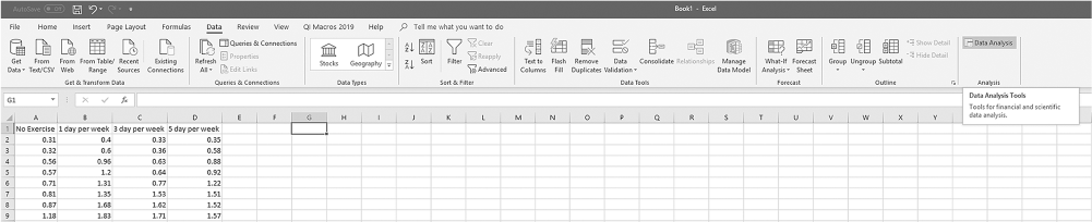
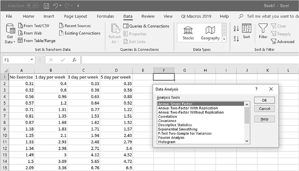
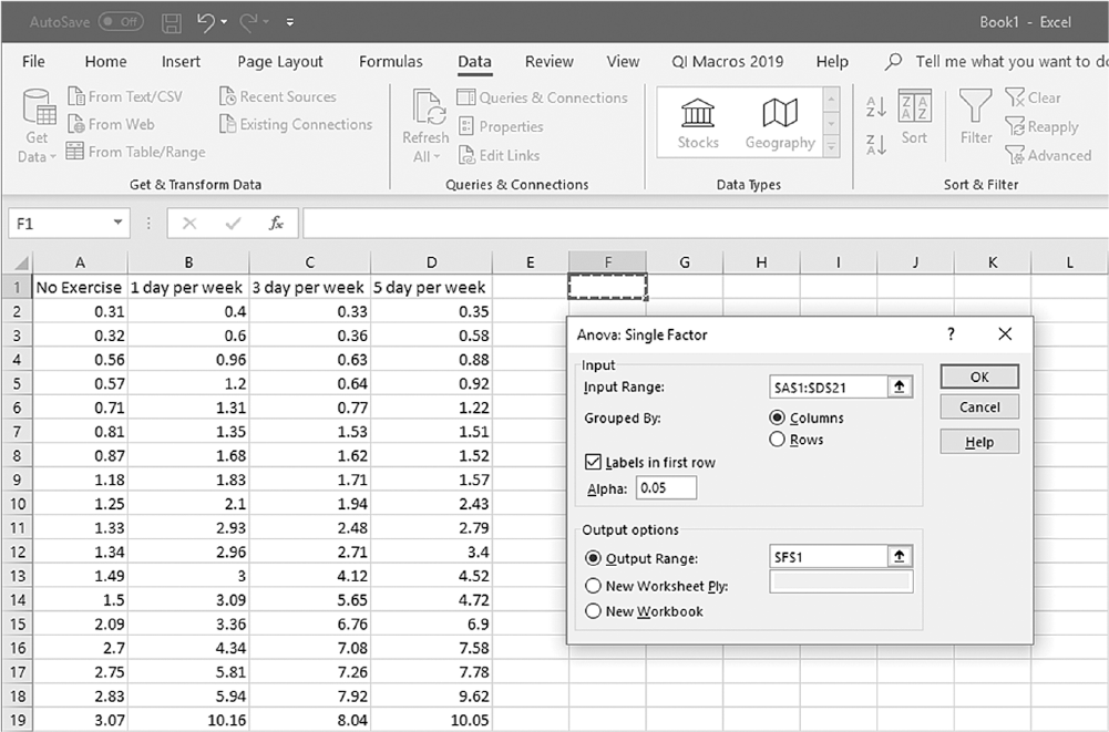
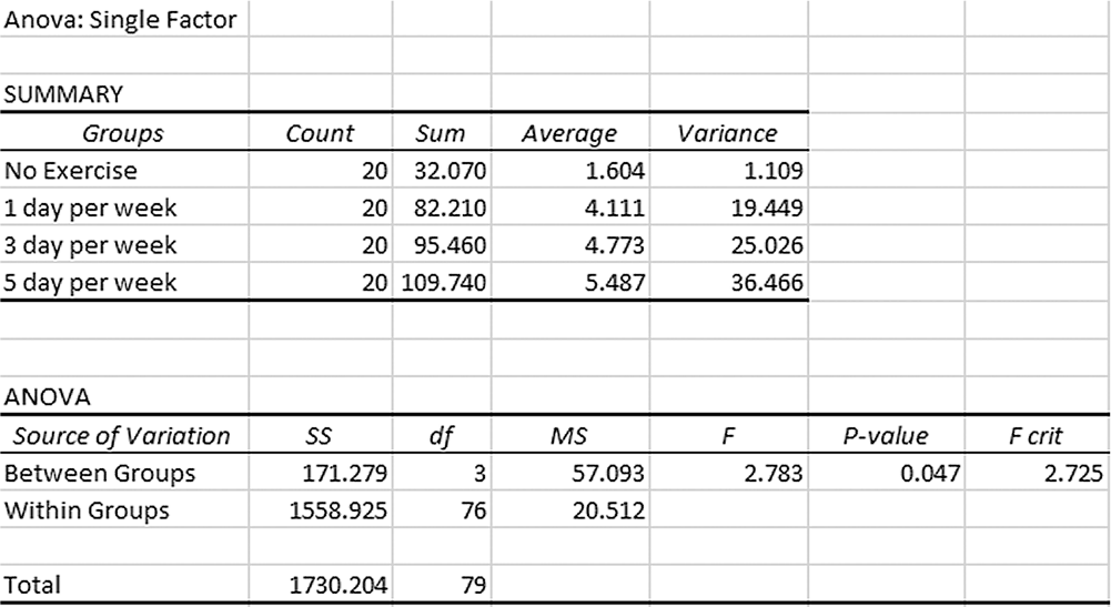
To conduct a one-way ANOVA in Excel, you will open Exercise.sav and go to Data > Data Analysis, as presented in Figure 12-27. In the Data Analysis window, choose "ANOVA: Single Factor" and then click "OK" (Figure 12-28). In the "ANOVA: Single Factor" dialogue box, you will provide A1:D21 as the Input Range and F1 as the Output Range with Labels in the First Row selected (Figure 12-29). Clicking "OK" will then produce the output of the requested ANOVA. The example output is presented in Figure 12-30.
Finding Data Analysis TookPak in Excel.
An Excel screenshot shows the Data Analysis ToolPak add-in, in the Analysis group under Data menu.
Courtesy of Microsoft Excel © Microsoft 2020.
Selecting "ANOVA: Single Factor" in Data Analysis Window in Excel.
An Excel screenshot shows selection of option, ANOVA: Single Factor, in the Data Analysis dialog box. The worksheet has four columns, No Exercise, 1 day per week, 3 day per week, and 5 day per week, with corresponding rows of data under each column.
Courtesy of Microsoft Excel © Microsoft 2020.
Defining input range and output range in "ANOVA: Single Factor" in Excel.
An Excel screenshot shows the ANOVA: Single Factor dialog box with fields to define data. The worksheet has four columns, No Exercise, 1 day per week, 3 day per week, and 5 day per week, with corresponding rows of data under each column.
The dialog box has two textboxes. The first textbox with heading, Input, consists of a drop-down list, input range; Grouped by with two options, Columns and Rows, preceded by option buttons, of which Columns is selected; and the text, Labels in first row, preceded by a check box which is checked. The second textbox with heading, Output options, consists of a drop-down list, output range which is checked and the cell F 1 entered; new worksheet ply; and new worksheet. The buttons, O k, Cancel, and Help, are on the right of the dialog box.
Courtesy of Microsoft Excel © Microsoft 2020.
Example output of ANOVA: Single Factor in Excel.
An Excel screenshot displays the output of ANOVA: Single Factor. There are two tables.
The heading of the first table reads, Summary. The output has five columns, Groups, Count, Sum, Average, and Variance. The row entries are as follows. Row 1: No Exercise, 20, 32.070, 1.604, 1.109. Row 2: 1 day per week, 20, 82.210, 4.111, 19.449. Row 3: 3 day per week, 20, 95.460, 4.773, 25.026. Row 4: 5 day per week, 20, 109.740, 5.487, 36.466. The heading of the first table reads, ANOVA. The output has seven columns, Source of variation, S S, d f, M S, F, p-value, and F crit. The row entries are as follows. Row 1: Between groups, 171.279, 3, 57.093, 2.783, 0.047, 2.725. Row 2: Within groups, 1558.925, 76, 20.512, no data, no data, no data. Row 3: Total, 1730.204, 79, no data, no data, no data, no data.
Courtesy of Microsoft Excel © Microsoft 2020.
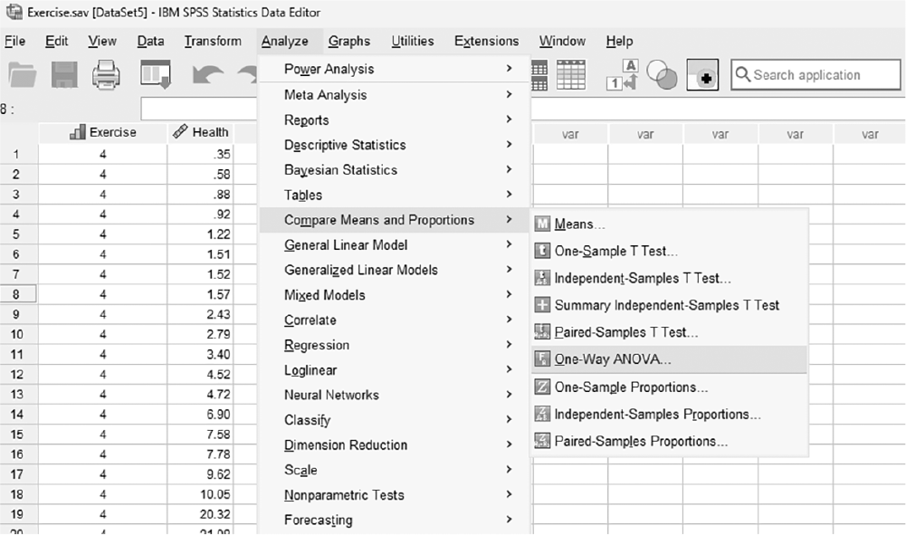
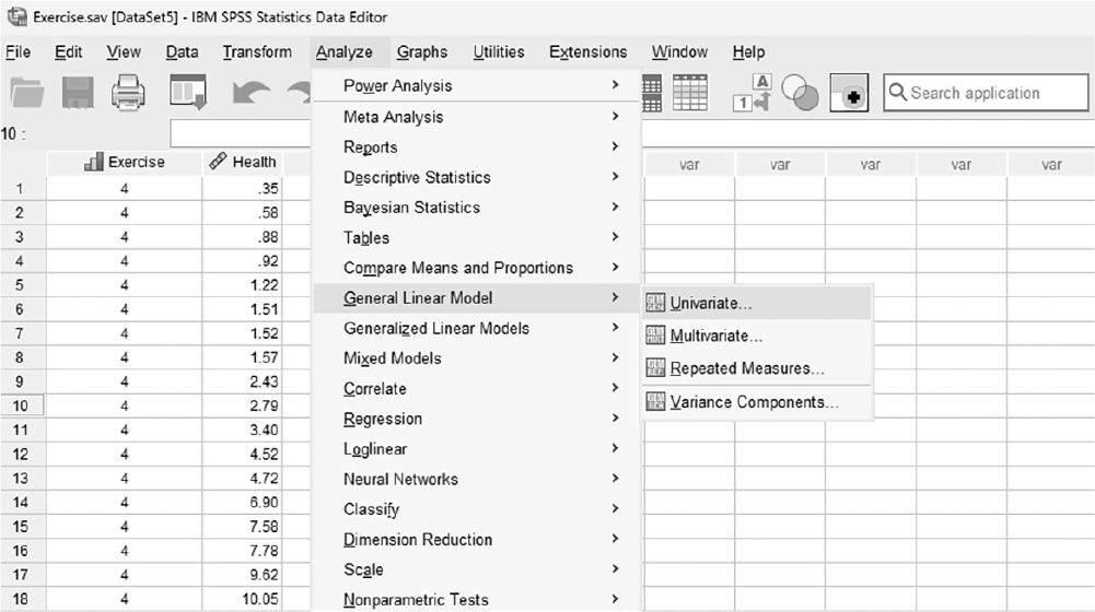
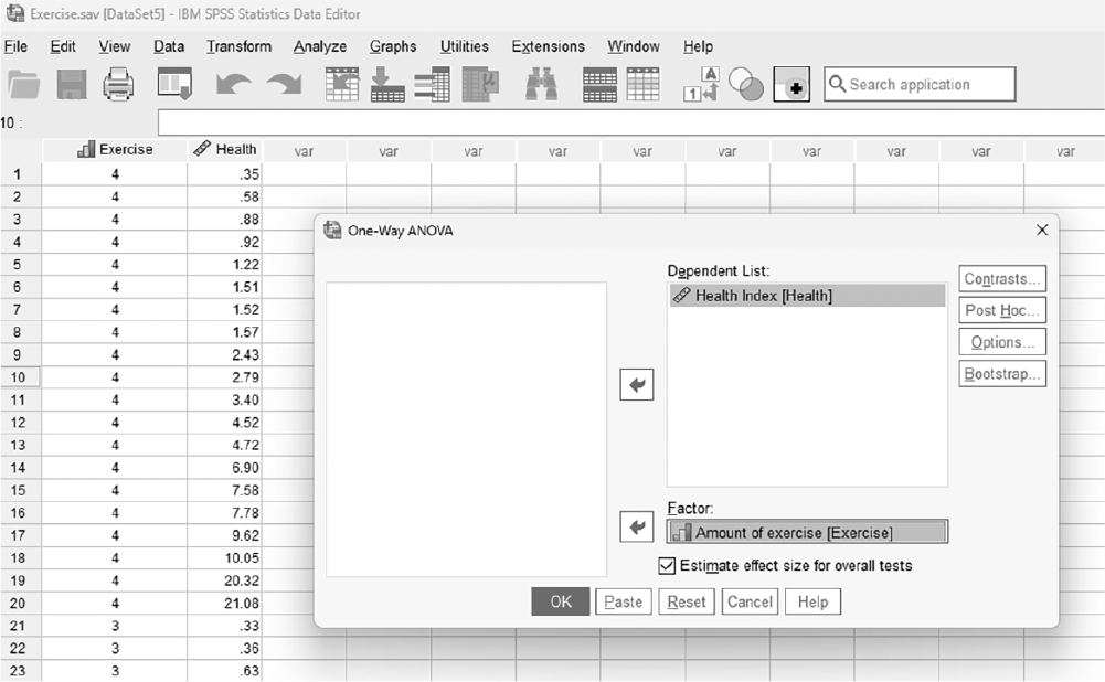
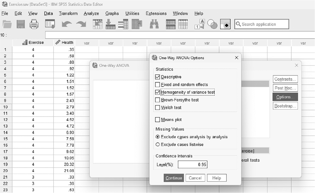
To conduct a one-way ANOVA in SPSS, you will open Exercise.sav and can go to either Analyze > Compare means > One-way ANOVA or Analyze > Generalized linear models > Univariate, as displayed in Figures 12-31 and 12-32, respectively. The data presented in the figures represent the amount of exercise as an independent variable and the health index as a dependent variable. We will first examine how to conduct one-way ANOVA in Analyze > Compare means > One-way ANOVA. In the One-Way ANOVA dialogue box, you will move an independent variable into "Factor" and a dependent variable into "Dependent List" by clicking the corresponding arrow buttons in the middle (refer to Figure 12-33). There are three buttons in the box; click on the "Options" button for now and check "Descriptives" and "Homogeneity of variance test" (refer to Figure 12-34). Clicking "Continue" and "OK" will produce the requested ANOVA analysis output. Example output is presented in Table 12-4.
Selecting one-way ANOVA under "Compare Means" in SPSS.
A screenshot displays a dialog box listing analysis procedures, with the One-Way ANOVA option highlighted under the Compare Means menu.
Reprint Courtesy of International Business Machines Corporation, © International Business Machines Corporation. "IBM SPSS Statistics software ("SPSS")". IBM®, the IBM logo, ibm.com, and SPSS are trademarks or registered trademarks of International Business Machines Corporation.
Selecting one-way ANOVA under "General Linear Models" in SPSS.
A screenshot displays a dialog box listing General Linear Model options, with the one-way ANOVA option highlighted for selection.
Reprint Courtesy of International Business Machines Corporation, © International Business Machines Corporation. "IBM SPSS Statistics software ("SPSS")". IBM®, the IBM logo, ibm.com, and SPSS are trademarks or registered trademarks of International Business Machines Corporation.
Defining variables in one-way ANOVA in SPSS.
A screenshot displays a dialog box where a dependent variable is placed in its designated field and a factor variable is assigned to the factor field.
Reprint Courtesy of International Business Machines Corporation, © International Business Machines Corporation. "IBM SPSS Statistics software ("SPSS")". IBM®, the IBM logo, ibm.com, and SPSS are trademarks or registered trademarks of International Business Machines Corporation.
Selecting options in one-way ANOVA in SPSS.
A screenshot displays a dialog box showing checkboxes and buttons for selecting post hoc tests, descriptive statistics, and other analysis options.
Reprint Courtesy of International Business Machines Corporation, © International Business Machines Corporation. "IBM SPSS Statistics software ("SPSS")". IBM®, the IBM logo, ibm.com, and SPSS are trademarks or registered trademarks of International Business Machines Corporation.
Descriptives | ||||||||
Health Index | ||||||||
95% Confidence lnterval for Mean | ||||||||
N | Mean | Std. Deviation | Std. Error | Lower Bound | Upper Bound | Minimum | Maximum | |
None | 20 | 1.6031 | 1.05270 | 0.23539 | 1.1104 | 2.0958 | 0.31 | 4.11 |
1 day per Week | 20 | 4.1101 | 4.40991 | 0.98609 | 2.0462 | 6.1740 | 0.40 | 18.21 |
3 days per Week | 20 | 4.7725 | 5.00301 | 1.11871 | 2.4310 | 7.1140 | 0.33 | 18.47 |
5 days per Week | 20 | 5.4866 | 6.03848 | 1.35025 | 2.6605 | 8.3127 | 0.35 | 21.08 |
Total | 80 | 3.9931 | 4.67988 | 0.52323 | 2.9516 | 5.0345 | 0.31 | 21.08 |
Tests of Homogeneity of Variances | ||||||||
Levene Statistic | df1 | df2 | Sig. | |||||
Health Index | Based on mean | 5.799 | 3 | 76 | 0.001 | |||
Based on median | 3.036 | 3 | 76 | 0.034 | ||||
Based on medianand with adjusted df | 3.036 | 3 | 54.285 | 0.037 | ||||
Based on trimmed mean | 4.708 | 3 | 76 | 0.005 | ||||
ANOVA | ||||||||
Health Index | ||||||||
Sum of Squares | df | Mean Square | F | Sig. | ||||
Between Groups | 171.276 | 3 | 57.092 | 2.783 | 0.047 | |||
Within Groups | 1558.928 | 76 | 20.512 | |||||
Total | 1730.203 | 79 | ||||||
ANOVA Effect Sizesa,b | ||||||||
95% Confidence lnterval | ||||||||
Point Estimate | Lower | Upper | ||||||
Health Index | Eta-squared | 0.099 | 0.000 | 0.211 | ||||
Epsilon-squared | 0.063 | μ0.039 | 0.180 | |||||
Omega-squared Fixed-effect | 0.063 | μ0.039 | 0.178 | |||||
Omega-squared Random-effect | 0.022 | μ0.013 | 0.067 | |||||
a. Eta-squared and Epsilon-squared are estimated based on the fixed-effect model. b. Negative but less biased estimates are retained, not rounded to zero. | ||||||||
You will notice that the health problem index for the "no exercise" group is 1.60, which seems to be lower than the index of the other three groups. The group that exercised once a week showed a health index of 4.11, the group that exercised 3 days per week had a health index of 4.77, and the group that exercised 5 days per week showed a health index of 5.49. So, is the difference among these four groups substantial enough to say that it is an effect of exercise?
Levene's test results for the homogeneity of variance assumption indicate that this assumption is violated. Recall that this test assumes the variances across the groups to be equal, so a small p-value of .001, as presented in Table 12-4, leads us to reject the null hypothesis, concluding that the variances are not the same. One thing to note here is that when the sample sizes across all groups are the same, one-way ANOVA is known to be robust to the violation of equal variances and normality. Therefore, we can somewhat ignore this violation.
The ANOVA table presents the F-statistic (this is the statistical test reflecting the F-distribution used in all ANOVAs) and the associated p-values of 2.783 and .047, respectively. Because the p-value of .047 is small enough to rule out chance, the null hypothesis is rejected and the health index is different between/among at least two exercise groups.
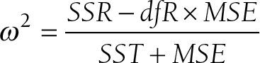
When reporting one-way ANOVA results, you should report the F-statistic, degrees of freedom, and associated p-value. The effect size for one-way ANOVA results is called omega squared (ω2) and is found with the following equation:

Formula reads: omega squared equals open parenthesis S S R minus d f R times M S E close parenthesis over open parenthesis S S T plus M S E close parenthesis.
where SSR is the sums of squares for regression, dfR is the degrees of freedom for regression, MSE is the mean squares for residual, and SST is the total sums of squares. Note that ω2 can only be calculated when the group sample sizes are equal.
The following is a sample report of our example.
There was a weak effect of the amount of exercise per week on health index, F (3, 76) = 2.78, p = .047, ω2 = .06.
If we had concluded that the amount of exercise did not make a difference on the health index and we decided not to reject the null hypothesis, then no further analysis would be needed. In our previous example, however, further analysis is needed because the amount of exercise made a substantial difference on the health index. Remember that a one-way ANOVA result with a small p-value does not necessarily indicate which of the groups differ. Therefore, we need to conduct further comparisons to find out exactly how the groups differ from each other; these analyses are called planned contrasts and post hoc tests.
Orthogonal planned contrasts, sometimes called a priori tests, are used when specific comparisons are determined before an examination of the data because you expect specific means to differ. These comparisons are often theory driven and protect us from overly increasing
Type I error. To set orthogonal planned contrasts, there are some rules to follow when choosing the theory-driven comparisons:
Rule #1: Groups that are included in the comparison get either positive or negative weights. Groups that have positive weights are compared with groups that have negative weights.
Rule #2: Groups that are excluded from the comparison get zero weights.
Rule #3: The sum of all weights in the comparison adds up to zero.
Recall that we found that the effect of the amount of exercise differed in our previous example, and we are specifically interested in whether exercising more than 3 days a week improves the health index. We then apply positive weights of +1 to 3 days per week and 5 days per week and negative weights of -1 to none and 1 day per week. These weights create orthogonal planned contrasts, as they sum up to zero.
Consider next that we are interested in whether exercising even 1 day per week improves the health index. We then apply a positive weight of +3 to none and negative weights of -1 to 1 day per week, 3 days per week, and 5 days per week. These weights sum up to zero, so they are orthogonal planned contrasts.
These examples of contrast weights are summarized in Table 12-5.
None | 1 Day per Week | 3 Days per Week | 5 Days per Week | |
|---|---|---|---|---|
Example 1 | -1 | -1 | +1 | +1 |
Example 2 | +3 | -1 | -1 | -1 |
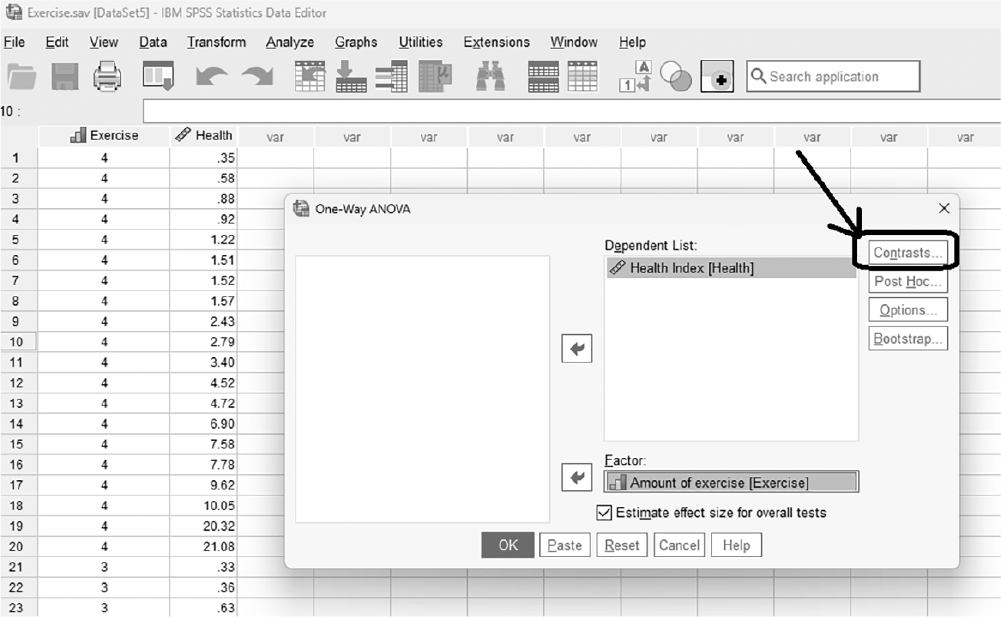
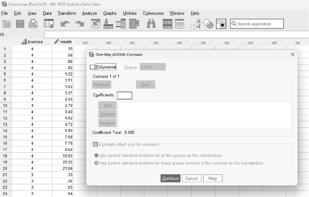
To conduct planned contrasts in SPSS, click on the "Contrasts" button in the One-Way ANOVA dialogue box, as presented in Figure 12-35; the One-Way ANOVA Contrasts dialogue box is displayed in Figure 12-36. Type the proposed coefficients in the One-Way ANOVA Contrasts dialogue box, in order, from the first group. For example, we would enter -1, -1, +1, and +1 in order for our first example and +3, -1, -1, and -1 for the second example. Note that you need to click on "Add" for each coefficient. Then, click "Continue" and proceed as you did with one-way ANOVA. This procedure will produce the output of requested planned contrasts. An example output for our first example is presented in Table 12-6. Results indicate that the mean health index for those who exercise 3 or 5 days per week is substantially higher than that for those who do not exercise or those who exercise only 1 day per week.
Selecting "Contrasts" in the One-Way ANOVA dialogue box in SPSS.
A screenshot displays the One-Way ANOVA dialog box with a button labeled Contrasts highlighted on the right side.
Reprint Courtesy of International Business Machines Corporation, © International Business Machines Corporation. "IBM SPSS Statistics software ("SPSS")". IBM®, the IBM logo, ibm.com, and SPSS are trademarks or registered trademarks of International Business Machines Corporation.
The One-Way ANOVA Contrasts dialogue box in SPSS.
A screenshot displays a dialog box with fields to specify contrast coefficients and buttons to add, delete, or reset contrast values.
Reprint Courtesy of International Business Machines Corporation, © International Business Machines Corporation. "IBM SPSS Statistics software ("SPSS")". IBM®, the IBM logo, ibm.com, and SPSS are trademarks or registered trademarks of International Business Machines Corporation.
Contrast Coefficients | |||||||||
|---|---|---|---|---|---|---|---|---|---|
Amount of Exercise | |||||||||
Contrast | None | 1 Day per Week | 3 Days per Week | 5 Days per Week | |||||
1 | μ1 | μ1 | 1 | 1 | |||||
2 | 3 | μ1 | μ1 | μ1 | |||||
Contrast Tests | |||||||||
95% Confidence Interval | |||||||||
Contrast | Value of Contrast | Std. Error | t | df | Sig. (2-Tailed) | Lower | Upper | ||
Health Index | Assumes equal variances | 1 | 4.5459 | 2.02545 | 2.244 | 76 | 0.028 | 0.5119 | 8.5800 |
2 | μ9.5599 | 3.50818 | μ2.725 | 76 | 0.008 | μ16.5470 | μ2.5727 | ||
Does not assume equal variances | 1 | 4.5459 | 2.02545 | 2.244 | 54.767 | 0.029 | 0.4865 | 8.6054 | |
2 | μ9.5599 | 2.13207 | μ4.484 | 64.527 | <.001 | μ13.8185 | μ5.3012 | ||
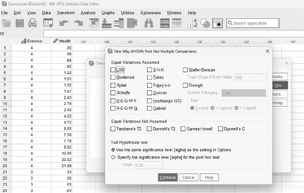
Post hoc tests are used when you want to make comparisons after examining the data to determine what means are contributing the greatest amount of variance by comparing all possible pairs of means. Note that the number of possible pairs to compare increases as the number of groups increases. For example, there are three tests of mean pairs when there are three groups (i.e., 1 vs. 2, 1 vs. 3, and 2 vs. 3). However, this number increases to six when there are four groups to compare pairwise (i.e., 1 vs. 2, 1 vs. 3, 1 vs. 4, 2 vs. 3, 2 vs. 4, and 3 vs. 4). Many post hoc tests control for inflated Type I error. Many post hoc tests are available; however, we will only discuss the most commonly used. As demonstrated in Figure 12-38, the post hoc tests are divided into two groups: those assuming homogeneity of variance and those not.
The first group comprises tests that assume homogeneity of variance; most post hoc tests fall into this group. The most commonly used tests are the Bonferroni test, the Tukey test, and the Scheffe test. All these tests take steps to control Type I error inflation caused by conducting many comparisons. Either the Bonferroni test or the Tukey test is good when the number of comparisons is low, but the Tukey test is better when the number of comparisons is high (i.e., the number of comparisons is five or more).
The second group is composed of tests that do not assume homogeneity of variance, so they are useful when this assumption is violated. There are four different tests, but Dunnett's C test is most commonly used for correcting the problem associated with Type I error.
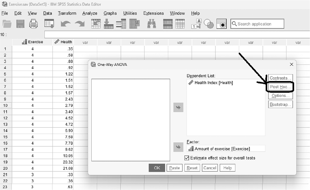
To conduct post hoc tests in SPSS, click on the "Post Hoc" button in the One-Way ANOVA dialogue box, as presented in Figure 12-37. The post hoc dialogue box is displayed in Figure 12-38; note that the two groups of post hoc tests are displayed. Select one of the post hoc tests in the dialogue box, depending on whether you violate the assumption of homogeneity of variance, and then click "Continue" to proceed as you did with one-way ANOVA. Note that we will use Dunnett's C test, as we violated the assumption of homogeneity of variance. This procedure will produce the output of requested post hoc tests. An example output is displayed in Table 12-7. Results indicate that those who exercise 5 days per week have a substantially higher health index than those who do not.
Selecting "Post Hoc" in the One-Way ANOVA dialogue box in SPSS.
A screenshot displays the One-Way ANOVA dialog box with a button labeled Post Hoc highlighted on the right side.
Reprint Courtesy of International Business Machines Corporation, © International Business Machines Corporation. "IBM SPSS Statistics software ("SPSS")". IBM®, the IBM logo, ibm.com, and SPSS are trademarks or registered trademarks of International Business Machines Corporation.
The Post Hoc dialogue box in SPSS.
A screenshot displays a dialog box listing post hoc test options with checkboxes beside each test name and a panel to select significance criteria.
Reprint Courtesy of International Business Machines Corporation, © International Business Machines Corporation. "IBM SPSS Statistics software ("SPSS")". IBM®, the IBM logo, ibm.com, and SPSS are trademarks or registered trademarks of International Business Machines Corporation.
Multiple Comparisons | |||||
|---|---|---|---|---|---|
Dependent Variable: Health Index | |||||
Dunnett C | |||||
95% Confidence lnterval | |||||
(I) Amount of Exercise | (J) Amount of Exercise | Mean Difference (I-J) | Std. Error | Lower Bound | Upper Bound |
None | 1 day per week | μ2.50696 | 1.01379 | μ5.3576 | 0.3437 |
3 days per week | μ3.16939 | 1.14320 | μ6.3839 | 0.0451 | |
5 days per week | μ3.88351a | 1.37061 | μ7.7375 | μ0.0296 | |
1 day per week | None | 2.50696 | 1.01379 | μ0.3437 | 5.3576 |
3 days per week | μ0.66242 | 1.49126 | μ4.8556 | 3.5308 | |
5 days per week | μ1.37655 | 1.67198 | μ6.0779 | 3.3248 | |
3 days per week | None | 3.16939 | 1.14320 | μ0.0451 | 6.3839 |
1 day per week | 0.66242 | 1.49126 | μ3.5308 | 4.8556 | |
5 days per week | μ0.71412 | 1.75347 | μ5.6446 | 4.2164 | |
5 days per week | None | μ3.88351a | 1.37061 | 0.0296 | 7.7375 |
1 day per week | 1.37655 | 1.67198 | μ3.3248 | 6.0779 | |
3 days per week | 0.71412 | 1.75347 | μ4.2164 | 5.6446 | |
a. The mean difference is significant at the 0.05 level. | |||||
Report planned contrasts results as you would with independent samples t-test results. The following is a sample report of our first planned contrast, where we compare groups that exercise 3 days or more per week against those who exercise fewer than 3 days.
Planned contrasts indicated that participants exercising 3 days or more per week have a higher health index than those who exercised fewer than 3 days per week, t(54.767) = 2.24, p = .029, r = .08.
When reporting post hoc test results, the p-value of each comparison along with the corresponding group descriptive statistics should be reported, such as in this example reporting of a Dunnett C post hoc test:
A Dunnett's C post hoc test indicates that there was a substantial difference on the health index between the group who do not exercise and the group who exercised 5 days per week, p< .05. The group who exercised 5 days per week had a higher index (M = 5.49, SD = 6.04) than the group who did not exercise (M = 1.60, SD =1.05), Cohen's d = .28, 95% CI [0.03, 7.74].
One-way ANOVA with planned contrasts combined with post hoc tests is a robust approach to testing hypotheses on a single dependent variable.
In this chapter, we have discussed how to conduct statistical tests that compare means. In nursing research, these tests are widely used to evaluate the effectiveness of treatments, compare patient outcomes, or assess differences across multiple populations. The simplest statistic for comparing two means is the t-test. The t-test and its variations allow us to compare two groups on a single dependent variable measured at the interval or ratio level. When we need to compare more than two groups and conserve power, we turn to analysis of variance. One-way ANOVA allows us to compare three or more groups on a single dependent variable. Planned contrasts and post hoc tests determine what groups contribute to the significance when an overall group difference is found.
All these techniques share similar assumptions related to normality, independence, and homogeneity of variance. Tests of differences between means are most useful in descriptive comparative and experimental designs in which the goal is often to identify the most effective interventions or understand variations in patient outcomes.
What statistical test would be most appropriate to examine differences between a sample mean and a population mean? Differences between men and women on exercise frequency? Differences between four ethnic groups on caloric intake?
What does "homogeneity of variance" mean in relation to conducting a one-way ANOVA?
How is the independent sample t-test different from the dependent sample difference test?
How would you decide whether to use a one-way ANOVA or multiple independent samples t-tests when comparing the means of more than two groups? What are the advantages and disadvantages of each approach?
What multiple comparison tests would be most helpful following an analysis of variance?
How does the number of groups influence the choice of a statistical test of difference?
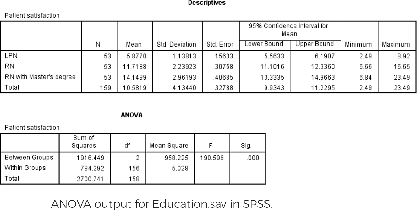
How would you report the following one-way ANOVA findings in APA style where an independent variable was nurses' education level?
How might you use the findings from the below ANOVA table in practice?
What are the potential limitations of using a t-test or ANOVA with small sample sizes, and how might this affect the reliability of the conclusions you draw?
How would you explain the difference between statistical significance and practical significance in the context of group mean tests?

An untitled 2-part table displays the A N O V A output for Education dot s a v in S P S S.
Table 1: Under Descriptives, under the sub-heading, Patient Satisfaction, the first part table displays the column-heads: N, Mean, Standard Deviation, Standard Error, Lower Bound under 95 percent Confidence Interval for Mean, Upper Bound under 95 percent Confidence Interval for Mean, Minimum, and finally Maximum. The row entries under these column heads in the above order for Row 1, L P N are as follows. 53, 5.8770, 1.13813, 0.15633, 5.5633 for Lower Bound, 6.1907 for Upper Bound, 2.49, and 8.92. Row 2 R N: 53, 11.7188, 2.23923, 0.30758, 11.1016 Lower Bound, 12.3360 Upper Bound, 6.66, and 16.65. Row 3 R N with Master's degree: 53, 14.1499, 2.96193, 0.40685, 13.3335 Lower Bound, 14.9663 Upper Bound, 6.84, and 23.49. Row 4 Total: 159, 10.5819, 4.13440, 0.32788, 9.9343 Lower Bound, 11.2295 Upper Bound, 2.49, and 23.49. Table 2: Under A N O V A, under the sub-heading, Patient satisfaction, the column heads are Sum of squares, d f, Mean Square, F, and Sig. The row entries are as follows under the above column heads in the same order: Row 1 Between Groups: 1916.449, 2, 958.225, 190.596, and point 000. Row 2 Within Groups: 784.292, 156, 5.028, Blank, and Blank. Row 3 Total: 2700.741, 158, Blank, Blank, and Blank.
Suppose you plan to compare SBP among three age groups: 50-65, 66-80, and 80 and older. What statistical test will be most appropriate?
One-way ANOVA
One-sample t-test
Independent t-test
Dependent t-test
You are planning to test the effect of music therapy on chronic pain intensity among a single group of older adults in long-term care. What statistical test will be appropriate to determine if a difference in pain intensity is present before and after treatment in a single group?
One-way ANOVA
One-sample t-test
Independent t-test
Dependent t-test
You find that there is a substantial mean difference among three different ethnic groups at risk of falls in a nursing home and want to find out which group differs specifically from which group. What procedure will help you determine such differences?
Skewness and/or kurtosis
Levene's test for homogeneity
Post hoc or planned contrast
What is the primary purpose of conducting post hoc tests?
To confirm the normality of the data
To identify which specific group means are different
To calculate the effect size
To check for outliers
True or False: In a one-way ANOVA, if the between-group variance is much larger than the within-group variance, it suggests that there may be significant differences between group means.
True of False: An effect size measures the magnitude of the difference between groups, regardless of sample size.
The Bonferroni correction is used to:
adjust the p-value for multiple comparisons
correct for violations of normality
increase the power of the test
test for interaction effects
True or False: A significant independent sample t-test result means that the two groups have exactly equal variances.
True or False: Post hoc tests are unnecessary if the one-way ANOVA results are not significant.
Which of the following scenarios would most likely require the use of a one-way ANOVA?
Comparing the average height of men and women.
Comparing the average blood pressure across four different age groups.
Comparing the pre- and post-test scores of the same group of students.
Comparing the effectiveness of two different medications.